The Taxonomy of Data

Types of variables and the data frame

Concept Acquisition

1. Data is a collection of measurements of variables made on observation units. They can be organized in a data frame.
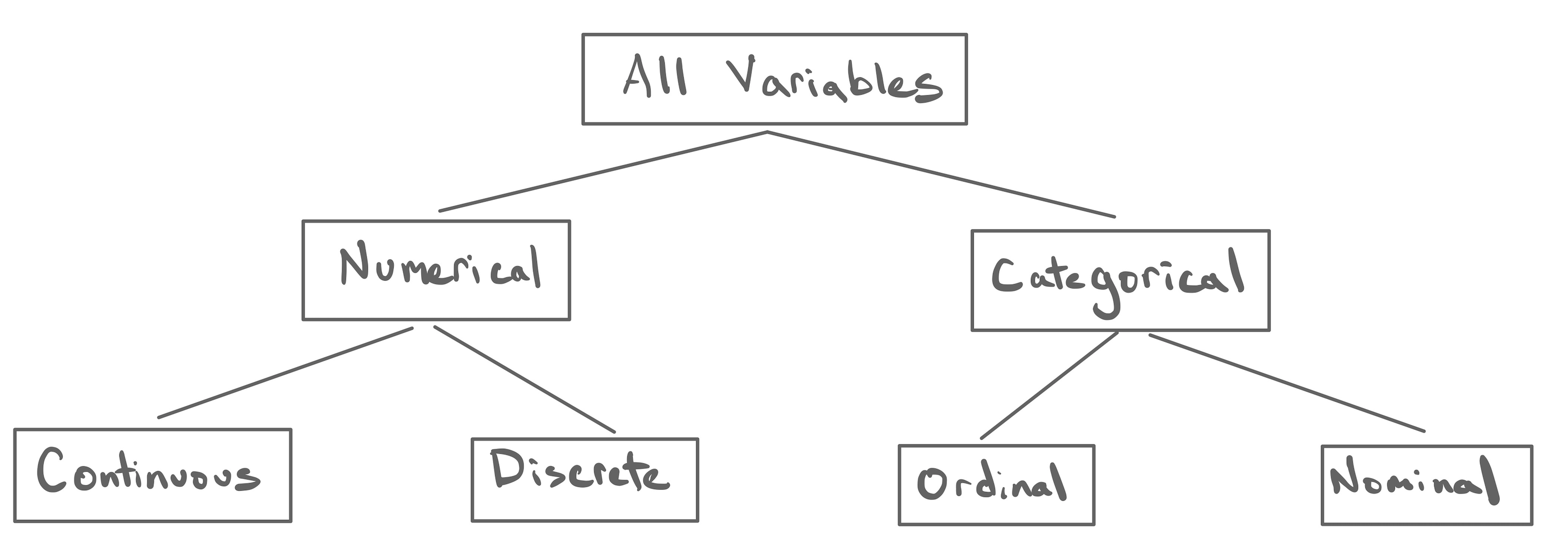
2. Variables can be classified as Numerical or Categorical. Types of numerical variables include continuous and discrete variables. Types of categorical variables include ordinal and nominal.

Tool Acquisition

1. Create a pdf document from a .qmd file using RStudio.

Concept Application

1. Identify the unit of observation in a written description of a study or in a given data frame.
2. Identify the variables recorded on the observations based on a written description of a study or in a given data frame. Classify each one according to the taxonomy of data.
3. Distinguish between a (tidy) data frame and other tabular displays.

---

Overview

In the beginning was data, and from that data was built an understanding of the world.

…or…

In the beginning was understanding, and from that understanding sprung questions that sought to be answered with data.

So, which is it?

This is a philosophical question and it is up for debate. What is clearer is that in the process of engaging in data science, you will inevitably find yourself at one of these beginnings, puzzling over how to make your way to the other one.

Figure 1: A big-picture view of what the Data Science Lifecycle.

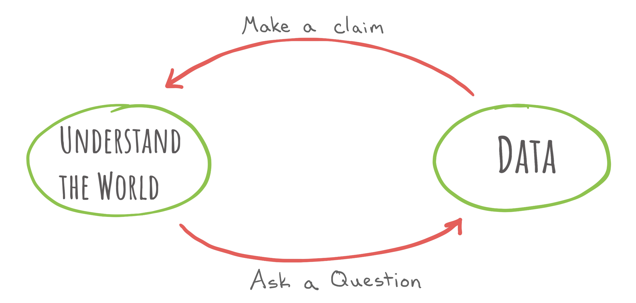
The defining element of data science is the centrality of data as the means of advancing our understanding of the world. The word “data” is used in many different ways, so let’s write down a definition to get everyone on the same page.

Data

• A piece of “data” is just a thing you know and wrote down. Someone’s name. The height of a giraffe. The temperature in Tulsa, Oklahoma at 3pm on July 19, 1987. You get it.
• The word comes from Latin datum: that which is given. Facts.
• So, data is “stuff we know already”. When a researcher goes to “gather data,” they are going out to find new facts and information to record (and later, study).

This broad definition permits a staggering diversity in the forms that data can take. When you conducted a chemistry experiment in high school and recorded your measurements in a table in a lab notebook, that was data. When you registered for this class and your name showed on CalCentral, that was data. When the James Webb Space Telescope took a photo of the distant reaches of our solar system, recording levels of light pixel-by-pixel, that was data.

Such diversity in data is more precisely described as diversity in the types of variables that are being measured in a data set.

Variable

• A “variable” is some kind of information you have on each of the “things” you are studying. So if we are studying penguins, a variable might be “species”. Some penguins are from the “Adelie” species, some are “Gentoo,” some are” Chinstrap,” etc. That is, the value of “species” will vary among penguins. Another variable could be “body mass” - again, each individual penguin has their own body mass, so “body mass” varies across penguins.
• Note: In writing computer code, a “variable” means something slightly different. We’ll talk more about this in the tutorial portion.

More examples:

• In your chemistry notebook you may have recorded the temperature and pressure of a unit of gas, two variables that are of scientific interest.
• In the CalCentral data set, name is the variable that was recorded (on you!) but you can imagine other variables that the registrars office might have recorded: your year at Cal, your major, etc.
• A psychiatrist studying depression might ask her patients how much they struggle with sleep on a 1-10 scale. This variable might be called “sleep difficulty.”

Again, things like “temperature” and “name” are called variables because each of the individuals in your dataset (people, penguins, whatever) may have different values for it. If we have a dataset of students in Stat 20, the name variable might have a value of “Penelope” for you and “Joaquin” for someone else.

A Taxonomy of Data

While the range of variables that we can conceive of is innumerable, there are recurring patterns in those variables that allow us to group them into persistent types that have shared properties. Such a practice of classification results in a taxonomy, which has been applied most notably in evolutionary biology to classify all forms of life.

Within the realm of data, an analogous taxonomy has emerged.

Figure 2: the Taxonomy of Data.

Types of Variables

Numerical vs Categorical

The principle quality of a variable is whether it is numerical or categorical.

Numerical Variable:

• A variable where the values are numbers with real quantitative meaning(see below).

• Not all numbers are numerical variables! The dividing line is: can you do useful math on it?
• Think about your cal student ID number. It’s definitely a number. But the fact that my number is 10 higher than your number by doesn’t mean anything. I couldn’t average a bunch of people’s Cal ID numbers and get anything useful.
• Same goes for phone numbers, area codes, etc. Doing math on these numbers is pointless. Hence, things like phone numbers and ID numbers are more like names – they are categorical (see below)
• Things like age, height, blood pressure, etc are** numerical variables.** Someone being “2 years older” than you, or having “a 10% faster reseting heartrate” than you can be useful. You can average a bunch of people’s ages to say something about how old the group is in general. Math means something on these variables, so they are numerical.

Categorical Variable:

Anything that is not numerical. Each unique value is called a level (see below).

Take “first name” for example. In a small class, maybe there is one student named Alice, two named Beckett, and three named Calista. This mini dataset might look like this:

student ID	name
1	Alice
2	Beckett
3	Beckett
4	Calista
5	Calista
6	Calista

name is a categorical variable here with three “levels”: Alice, Beckett, and Calista.

Other categorical variables are things like “species” in penguins, “home address” of people, and so forth. Remember, some numbers are categorical. As explained above, your student ID number, phone number, zip code, etc are not numerical variables despite being numbers.

Sub-types of numerical and categorical variables

• Numerical variables can be continuous or discrete
• Categorical variables can be nominal or ordinal

Types of numerical variables:

Continuous Numerical Variable: - Values can take any decimal number, though possibly in a restricted range.

Everyone’s feet are slightly different sizes. If you measure the length of your foot, maybe you’ll find that it’s about 9.5 inches long. But your foot is almost certainly not exactly 9.5 inches – that’s just the best approximation you could measure with your ruler. Your “real” foot length might be 9.5531 inches, or 9.472 inches. But 9.5 is as close as you can guess with your ruler, and in most cases that’s fine. Also you’re foot can’t be less than 0 inches, and no human has ever had a foot that is 100 inches long, so there’s a range. So “foot size” is continuous.

Other continuous numerical variables include the air temperature, wind speed, height of a mountain, etc. When we measure these, we have to round off to some number of decimals. It’s usually good enough to know that the wind speed is 12 mph – we don’t usually care that it’s actually 12.010935897 mph. Fancier measuring instruments might get us more decimal places of precision, but even the finest tools can’t capture the infinite range that wind speed can take in nature.

Discrete Numerical Variable:

A numerical variable that takes values that have jumps between them.

Shoe sizes are a great example here. Your foot size is continuous, but shoes don’t come in every possible length. If your foot is 9 inches long, that would be close to a women’s size 6.5, but not exactly. They don’t sell a size 6.51867 or whatåever would be literally perfect for you. Since shoe sizes are discrete, you have to make do with one that is close-enough to your foot size.

(Size chart for women’s shoes)

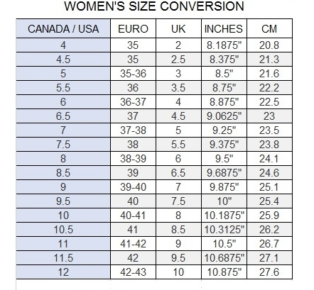
Another good discrete numerical variable is household size. When the US Census goes door-to-door every year collecting data on every household, they record the number of people living in that household. A household can have 1 person, or 2 people, or 3 people, or 4 people, and so on, but it cannot have 2.83944 people. This makes it discrete.

What unites both types of numerical variables is that the you can perform mathematical operations on them and the result has meaning. It is possible and meaningful to talk about the average air temperature across three locations. It is also possible and meaningful to talk about the sum total number of people across ten households. Or the average household size. But it’s not meaningful to average everyone’s area code, so area code is categorical.

Types of categorical variables:

Nominal Categorical Variable

• A categorical variable with levels with no natural order.
• “Name” is a good one. OK yes, often we order them alphabetically when we make a list of people, but that’s just to it easier to read. It’s not really true that the name “Alice” is “less than” the name “Bob.”

• Other good examples are home addresses, birds’ colors, people’s blood types, etc.
• Note that there are only four possible “blood types” (A, B, O, or AB), so we say that “blood type” has four levels.¹

¹Blood type is actually a fascinating concept and extends well beyond the A/B/O group. Check it out. These other blood types also matter in medicine, especially for things like organ transplants.

Ordinal Categorical Variable

• A categorical variable with levels that have a natural order.
• For example, a company might sell a T-shirt in three sizes: small, medium, and large. You can’t really average a bunch of t shirt sizes, but “small” is definitely less than “medium,” which is definitely less than “large.”

You have likely come across ordinal categorical variables if you have taken an opinion survey. Consider the question:“Do you strongly agree, agree, feel neutral about, disagree, or strongly disagree with the following statement: Dogs are better than cats?” When you record answers to this question, you’re recording measurements on a categorical variable that takes values “strongly agree”, “agree”, “neutral”, “disagree”, “strongly disagree”. Those are the levels of the categorical variable and they have a natural ordering: “strongly agree” is closer to “agree” than it is to “strongly disagree”.

Similarly, “infant,” “toddler,” “kid,” “teenager,” “adult,” and “senior” are common ways we refer to someone’s general age range. Clearly all “infants” are younger than all “toddlers” and so forth (there is a natural ordering), but the gaps between the steps may not be even. Going from infant to toddler takes about 2 years. Going from adult to senior might take 50 years.

You can contrast this with a nominal categorical variable. Consider a second question that asks (as the registrar does): “What is your name?” There are many more possible levels in this case - “Penelope”, “David”, “Shobhana”, etc. - but those levels have no natural ordering. In fact, this is very appropriate example of a nominal variable because the word itself derives from the Latin nomen, or “name”.

Let’s take a look at a real data set to see if we can identify the variables and their types.

Example: Palmer Penguins

Dr. Kristen Gorman is a fisheries and wildlife ecologist at the University of Alaska, Fairbanks whose work brought her to Palmer Station, a scientific research station run by the National Science Foundation in Antarctica. At Palmer Station, she took part in a long-term study to build an understanding of the breeding ecology and population structure of penguins.

Figure 3: Dr. Gorman recording measurements on penguins and Palmer Station, a research station in Antarctica.

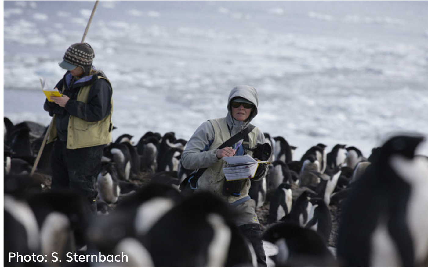
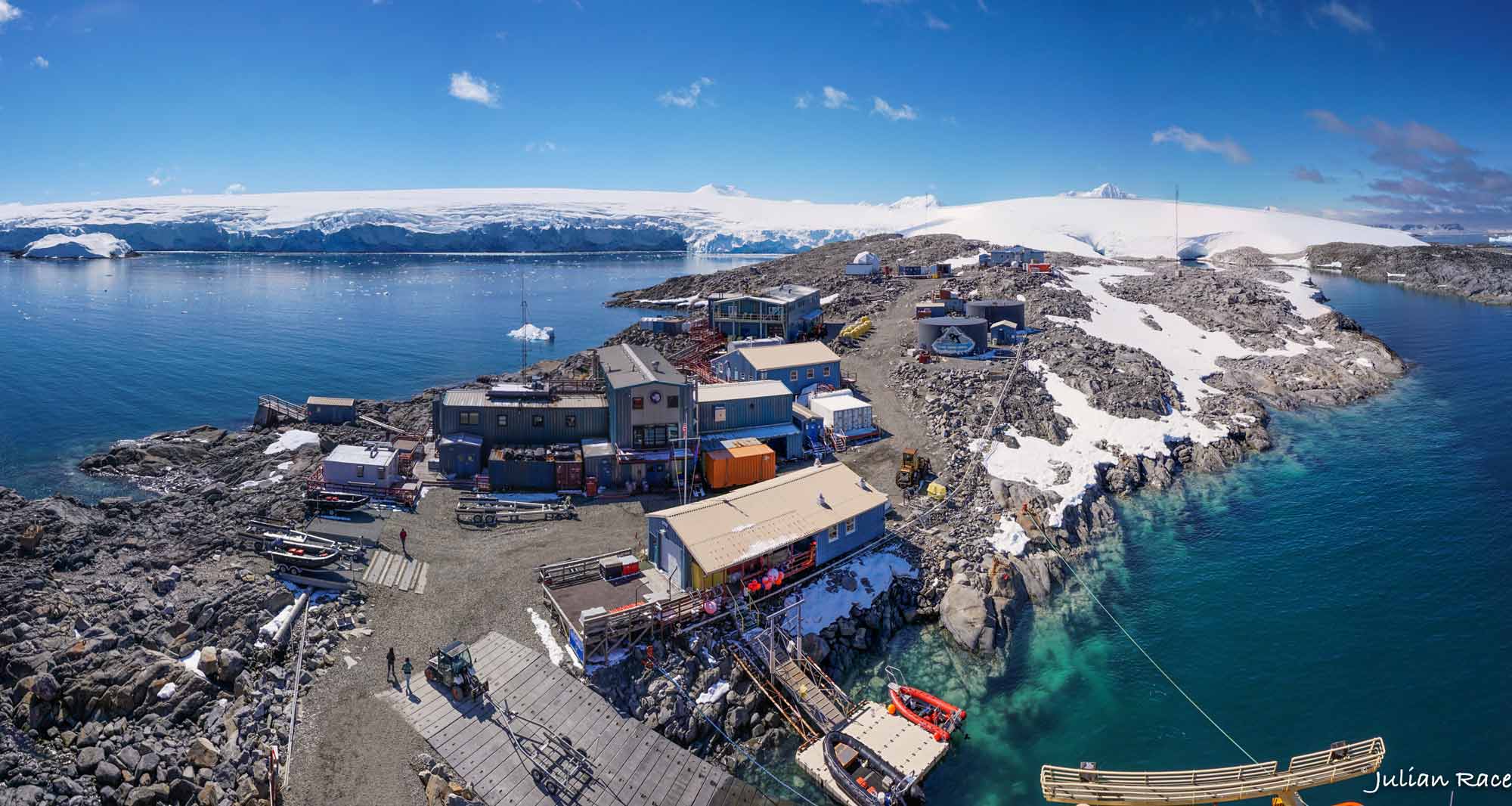
In order to build her understanding of this community of penguins, she and fellow scientists spent time in the field recording measurements on a range of variables that capture important physical characteristics.

Here is an excerpt of what her dataset looks like:

species	island	bill_length_mm	bill_depth_mm	flipper_length_mm	body_mass_g
Adelie	Biscoe	37.9	18.6	172	3150
Chinstrap	Torgersen	39.1	18.7	181	3750
Gentoo	Dream	40.8	18.9	208	4300
Adelie	Biscoe	45.3	13.7	210	4300
Gentoo	Biscoe	50.5	15.9	222	5550

Each row represents one penguin (our “unit of observation”). Each column is a variable.

Try to identify the specific variable type for each column above

click to show answer

The first two columns (species and island) are nominal categorical, while the next four are continuous numerical.

The species of a penguin is either “Adelie”, “Gentoo”, or “Chinstrap”. Because these values are not numbers, this is a categorical variable. More specifically, it’s a nominal categorical because there is no obvious natural ordering between these three species. Adelie isn’t “less than” Chinstrap or Gentoo.

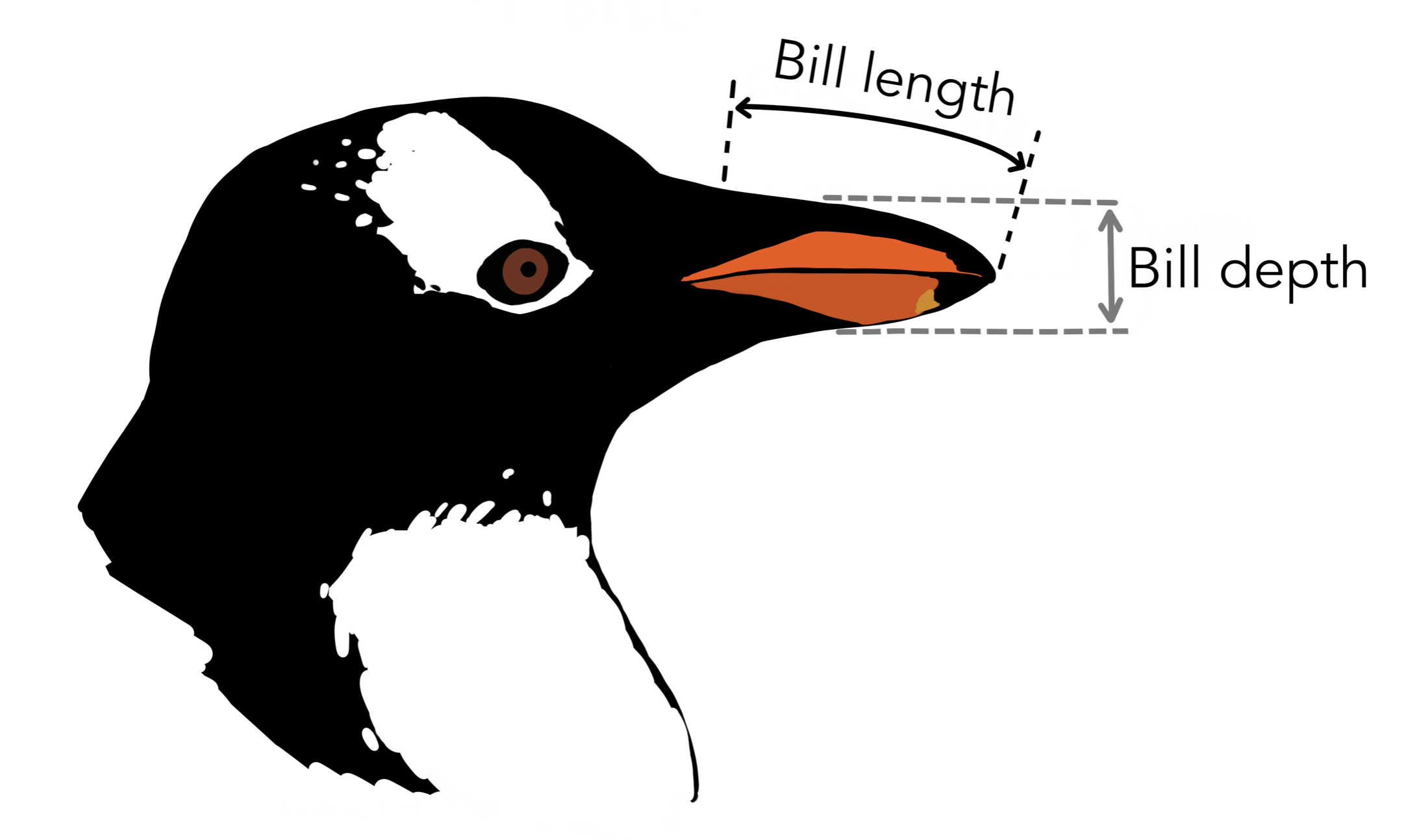
Two of the variables that were recorded were bill length and bill depth in millimeters (mm)¹. Each of these capture a dimension of the bill of a penguin. These are identifiable as continuous numerical variables. They’re numerical because the values have quantitative meaning (we can compare, subtract, and average them) and they’re continuous because bill sizes don’t come in fixed, standard increments. They are rounded off when written down, but true bill sizes vary continuously.

For more practice, see this week’s extras. Specifically, Data types and data frames

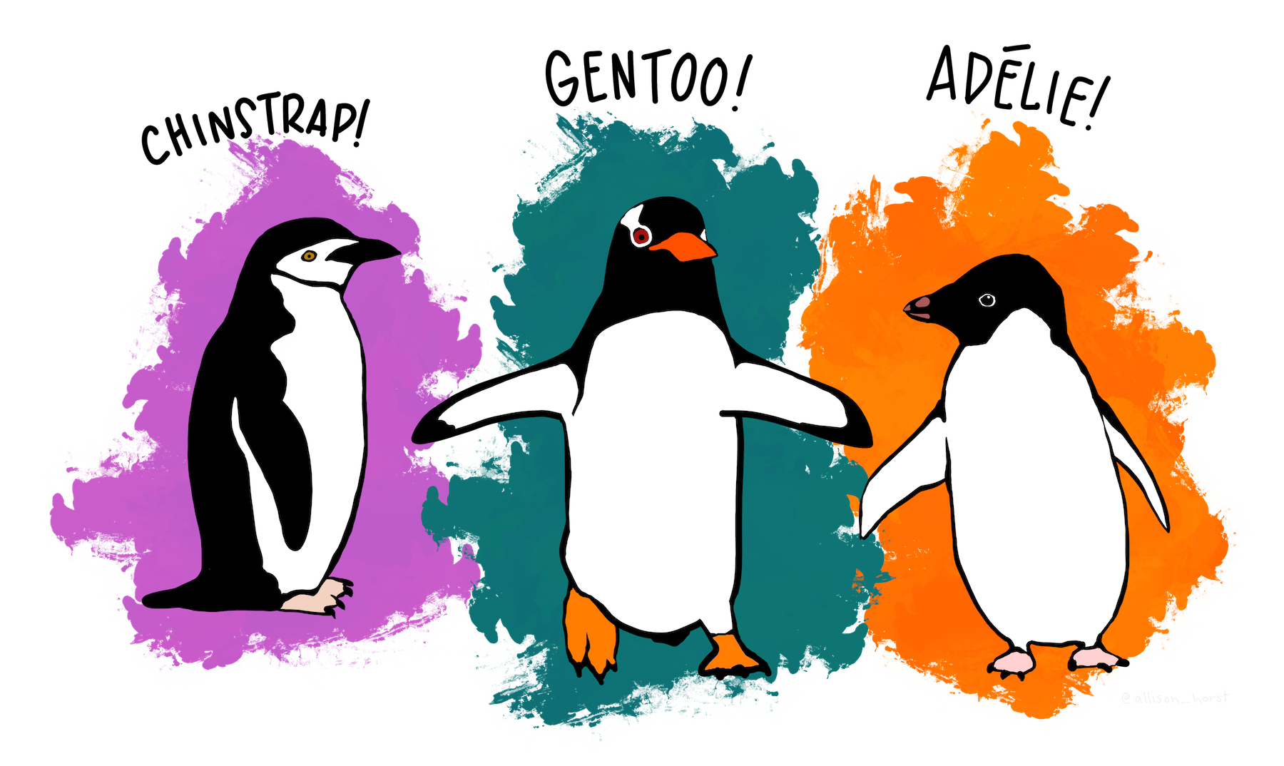
These are just three of many variables that recorded in the penguins data set and published along their scientific findings in the paper, Ecological sexual dimorphism and environmental variability within a community of Antarctic penguins (genus Pygoscelis)². We will return throughout this course to this data set and this study. It is a prime example of how careful data collection and careful scientific reasoning can expand our understanding of a corner of our world about which we know very little.

Why Types Matter

The Taxonomy of Data is a useful tool of statistics and data science because it helps guide the manner in which data is recorded, visualized, and analyzed. Many confusing plots have been made by not thinking carefully about whether a categorical variable is ordinal or not or by mistaking a continuous numerical variable for a categorical variable. You will get plenty of practice using this taxonomy to guide your data visualization in the next unit.

Like many tools built by scientists, this taxonomy isn’t perfect. There are many variables that don’t quite seem to fit into the taxonomy or that you can argue should fit into multiple types. That’s usually a sign that something interesting is afoot and is all the more reason to think carefully about the nature of the variables and the values it might take before diving into your analysis.

A Structure for Data: The Data Frame

When we are trying to study something in the world, sometimes we select a single variable that we go out and collect data on. More often, we’re dealing with more complex phenomenon that are characterized by a few, or a few dozen, or hundreds (or even millions!) of variables. CalCentral has far more than just your name on file. To capture all of the complexity of class registration at Cal, it is necessary to record dozens of variables.

To keep all of this data organized, we need a structure. While there are several different ways to structure a given data set, the format that has become most central to data science is the data frame.

Data Frame

• An table that associates the observations (rows) with the variables measured on each observation (columns).

The penguins table shown earlier is an example. We are studying penguins (our “unit of observation”), so a given row has all the information about one penguin. Each cell in that row stores that penguin’s value of a specific variable. Let’s bring that penguin table back to drive it home:

species	island	bill_length_mm	bill_depth_mm	flipper_length_mm	body_mass_g
Adelie	Biscoe	37.9	18.6	172	3150
Chinstrap	Torgersen	39.1	18.7	181	3750
Gentoo	Dream	40.8	18.9	208	4300
Adelie	Biscoe	45.3	13.7	210	4300
Gentoo	Biscoe	50.5	15.9	222	5550

We’ve got five penguins here. The first one (first row) is an Adelie penguin, who lives on Biscoe island, has a bill that is 37.9mm long and 18.6mm deep, has flippers that are 172mm long, and weighs 3150 grams (so about three kilos, or 6.5 pounds).

We could also read down a column. We’ve got five penguins: 3 from Biscoe Island, 1 from Dream Island, and one from Torgersen Island.

You might be accustomed to calling this a “spreadsheet” or a “table”, but the organizational norm of putting the variables down the columns and the observations across the rows make this a more specific structure.

One of the first questions that you should ask yourself when you first come across a data frame is this: “What is the unit of observation?”

Unit of Observation

• The “things” we are studying. If it’s a true dataframe, each row is exactly one observation. So the “unit of observation” is just “what does a single row represent?”

In the case of the penguins data frame above, the unit of observation is a single penguin (observed by the researchers in this study). The first row captures the measurements on the first penguin, the second row captures the measurements of the second penguin, and so on.

If I log into CalCentral to see the data frame that records information on the students enrolled in this class, the unit of observation is a single student enrolled in this class. There may be many variables on each student, each tracked in a column (things like name, year in school, etc).

Not a Data Frame

Before you leave thinking that “data frame” = “spreadsheet”, consider this data set:

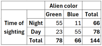
This may be a useful table, but it is not a dataframe. Let’s talk about why.

First, what are these researchers studying? Aliens. Specifically, alien sightings. When they see an alien, they’re recording its color and when it was seen. In a true data frame, there would be one row per alien sighting, with two columns: “color” and “time of sighting.” With 144 alien sightings, we should have 144 rows.

That’s not what we see here. The first row is not an observation at all, but the total number of observations, at night, of aliens of various colors. There are 66 total observations (alien sightings) packed into one row! That’s not a dataframe.

Instead, this is a summary table of some kind, built from the initial dataframe of 144 sightings, to produce an overview that is useful to understand what’s going on.

More practice

See this week’s extras. Specifically, Data types and data frames

Summary

In this lecture note we have focused on the nature of the data that will serve as the currency from which we’ll construct an improved understanding of the world. A first step is to identify the characteristics of the variables that are being measured and determine their type within the Taxonomy of Data. A second step is to organize them into a data frame to clearly associate the value that is measured for a variable with a particular observational unit.

With these ideas in hand, we learned how to bring data onto our computer, so that in our next class, we can begin the process of identifying its structure and communicating that structure numerically and visually.

Continue on to the tutorial portion of the notes

Footnotes

1. Penguin artwork by @allison_horst.

2. Gorman KB, Williams TD, Fraser WR (2014). Ecological sexual dimorphism and environmental variability within a community of Antarctic penguins (genus Pygoscelis). PLoS ONE 9(3):e90081. https://doi.org/10.1371/journal.pone.0090081