- the techniques we need to actually compute probabilities:
- probabilities of intersections using conditional probabilities
- what are independent events
- the difference between mutually exclusive and independent events
- inclusion-exclusion formula
Concept Acquisition
- Conditional probability & multiplication rule
- Independence
- Mutually exclusive events vs independent events
Concept Application
- Computing probabilities in various scenarios
- Using R to simulate probabilities
Sally Clark: a tragic victim of statistical illiteracy
In November 1999, Sally Clark, an English solicitor, was convicted of murdering her infant sons. The first, Christopher, had been 11 weeks old when he died, in 1996, and the second, Harry, 8 weeks old, in January 1998, when he was found dead. Christopher was believed to have been a victim of “cot death”, called SIDS (Sudden Infant Death Syndrome) in the US. After her second baby, Harry, also died in his crib, Sally Clark was arrested for murder. The star witness for the prosecution was a well known pediatrician and professor, Sir Roy Meadow, who authored the infamous Meadow’s Law :“One sudden infant death is a tragedy, two is suspicious and three is murder until proved otherwise”. Unfortunately it was easier to comprehend this “crude aphorism” than make the effort to understand the subtleties of conditional probability. The Royal Statistical Society protested the misuse of statistics in courts, but not early enough to prevent Sally Clark’s conviction. She was eventually acquitted and released, only to die at the age of 42 through alcohol poisoning The math presented by Meadow, in brief: Based on various studies, there is a probability of 1 in 8,543 of a baby dying of SIDS in a family such as the Clarks. As the Clarks suffered two deaths, Meadow multiplied 8,543 by 8,543 to arrive at 73 million. He told the jury that the chance or probability that the event of two “cot deaths” was 1 in 73 million. The defense did not employ a statistician to refute his claim, a choice that may have been disastrous for Sally Clark. Disastrous because the math was wrong, and the consequences tragic. Meadow multiplied probabilities that should not have been multiplied. This chapter tells us why.
We will revisit this case at the end of these notes to examine the mistake made by Sir Roy Meadow. How did such a brilliant man make such a terrible mistake? He wasn’t alone. Probability computations are easily mistaken, and we need to proceed carefully. Now, in order to understand why he was wrong, we need some more definitions.
Let’s go back to one of the examples with die rolls that we have seen, the outcomes that so puzzled and frustrated our seventeenth century gambler, the Chevalier De Méré.
Simulating De Méré’s dice games.
Recall that De Méré wanted to bet on at least one six in four rolls of a fair die, and also at least one double six in twenty-four rolls of a pair of dice.
In earlier notes, you have seen the result of simulating these two games to estimate the probability of De Méré winning his bet. The simulation used the idea of thinking of the probability of an event as the long-run relative frequency, or the proportion of times we observe that particular event (that is, we observe the outcomes in that event) if we repeat the action that can result in the event over and over again. Let’s do that again - that is, we estimate the probabilities using the long-run proportions. We will simulate playing the game over and over again and count the number of times we see at least one six in four rolls, and similarly for the second game. (De Méré did this by betting many times, and noticed that the number of times he won wasn’t matching the probability he had computed. Long-run relative frequency in real life!)
Number of simulations for game 1 (4 rolls of a die): 10000
The chance of at least one six in 4 rolls of a die is about 0.5156
Number of simulations for game 2 (24 rolls of a pair of dice): 10000
The chance of at least one double-six in 24 rolls of a pair of dice is about 0.4923
Now the question is how do we figure out this probability without simulations?
We know that if two events are mutually exclusive, we can compute the probability of at least one of the events occurring (\(A\cup B\) aka \(A \text{ or } B\)) using the addition rule \(P(A \cup B) = P(A) + P(B)\). We cannot use the addition rule to compute the probabilities that we have simulated above, since rolling a six on the first roll and rolling a six on the second roll (for example) are not mutually exclusive. So how do we compute the probability? Read on…
Example: Drawing red and blue tickets from a box
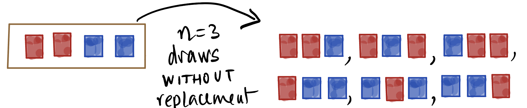
Consider a box with four tickets in it, two colored red and two blue. Except for their color, they are identical: 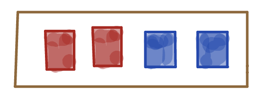 . Suppose we draw three times at random from this box, with replacement, that is, every time we draw a ticket from the box, we put it back before drawing the next ticket. List all the possible outcomes. What is the probability of seeing exactly 2 red cards among our draws?
Check your answer
Note that since each of the cards, and in particular, each of the two colors, is equally likely to be drawn, therefore all the sequences of colors in the three cards are equally likely. We can count the number of possible outcomes that contain exactly 2 red cards, and divide that number by the number of total possible outcomes to get the probability of drawing exactly 2 red cards:
 There are three outcomes that have exactly two red cards, out of a total of 8 possible outcomes, so the probability of exactly two red cards in three draws at random with replacement is 3/8.
Now suppose we repeat the procedure, but draw without replacement (we don’t put any tickets back). What is the probability of exactly 2 red cards in 3 draws?
Check your answer
Notice that we have fewer possible outcomes (6 instead of 8, because the number of possible outcomes reduces when we don’t put the drawn cards back), though they are still equally likely. Again, there are 3 outcomes that have exactly 2 red cards, and so the probability of 2 red cards in three draws is now 3/6. In this example, the six card sequences just so happen to have equal probabilities. When we draw without replacement, this is not always true,as you will see in the next example.”
What about the probabilities for the number of red cards in three draws? Write down all the possible values for the number of red cards in three draws from a box with 2 red cards and 2 blue cards, while drawing with replacement, and their corresponding probabilities. Repeat this exercise for the same quantity (number of red cards in three draws from a box with 2 red cards and 2 blue cards), when you draw the tickets without replacement:
Check your answer
| 0 red tickets |
\(\displaystyle \frac{1}{8}\) |
\(0\) |
| 1 red ticket |
\(\displaystyle \frac{3}{8}\) |
\(\displaystyle \frac{3}{6}\) |
| 2 red tickets |
\(\displaystyle \frac{3}{8}\) |
\(\displaystyle \frac{3}{6}\) |
| 3 red tickets |
\(\displaystyle \frac{1}{8}\) |
\(0\) |
Why are the numbers different? What is going on?
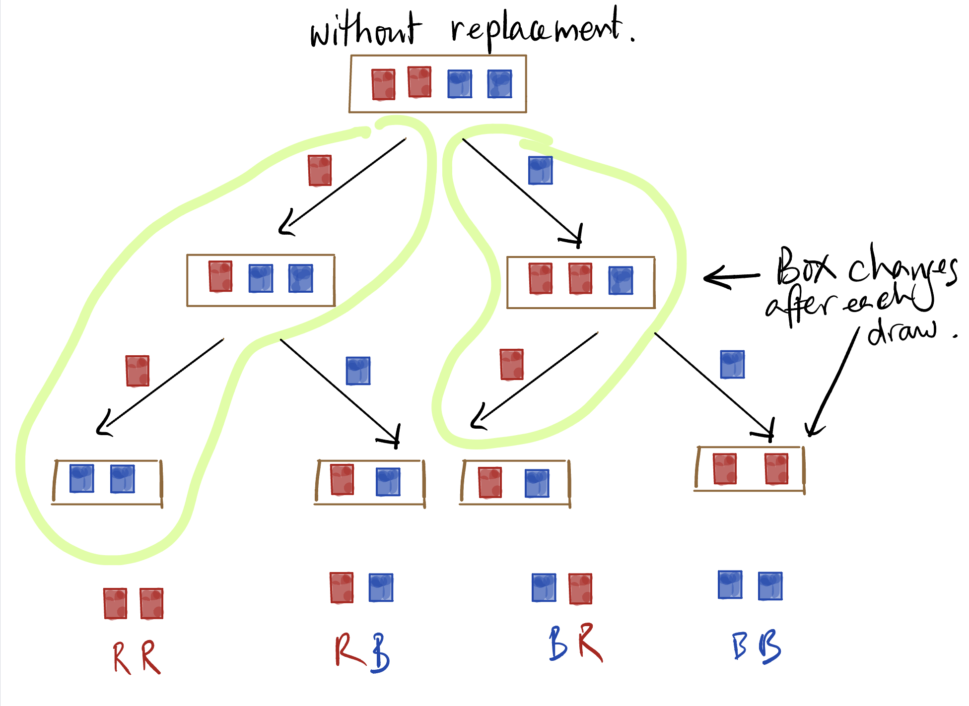
Below you see an illustration of what happens to the box when we draw without replacement, with the box at each stage being shown with one less ticket.
We see that the box reduces after each draw. After two draws, if the first 2 draws are red (as on the left most sequence) you can’t get another red ticket, whereas if you are drawing with replacement, you can keep on drawing red tickets. (Note that the outcomes in the bottom row are not equally likely, since on the left branch of the tree, blue is twice as likely as red to be the second card, so the outcome RB is twice as likely as RR, and the outcome BR on the right branch of the tree is twice as likely as BB.) Before going further, let’s recall what we know about the probabilities of events.
Rules of probability (recap)
\(\Omega\) is the set of all possible outcomes.
What is the probability of \(\Omega\)?
The probability of \(\Omega\) is 1. It is called the certain event.
When an event has no outcomes in it, it is called the impossible event, and denoted by \(\emptyset\) or \(\{\}\).
What is the probability of the impossible event?
The probability of the impossible event is 0.
Let \(A\) be a collection of outcomes (for example, from the example above, \(A\) could be the event of two red tickets in 3 draws with replacement).
Then the probability of \(A\) has to be ______ (fill in the blank with a suitable phrase)
between \(0\) and \(1\) (inclusive of \(0\) and \(1\)).
If \(A\) and \(B\) are two events with no outcomes in common,
then they are called ______ (fill in the blanks with suitable phrases)
mutually exclusive
If \(A\) and \(B\) have no outcomes in common, that is, \(A \cap B = \{\}\), then \(P(A \cup B) = P(A) + P(B)\).
Consider an event \(A\). The complement of \(A\) is not \(A\), and denoted by \(A^C\). The complement of \(A\) consists of all outcomes in \(\Omega\) that are not in \(A\) and \(P(A^C) = 1-P(A)\). (Why?)
Conditional probabilities
In the first example above, we saw that the probability of a red ticket on a draw changes if we sample without replacement. If we get a blue ticket on the first draw, the probability of a red ticket on the second draw is 2/3 (since there are 3 tickets left, of which 2 are red). If we get a red ticket on the first draw, the probability of a red ticket on the second draw is 1/3. These probabilities, that depend on what has happened on the first draw, are called conditional probabilities. If \(A\) is the event of a blue ticket on the first draw, and \(B\) is the event of a red ticket on the second draw, we say that the probability of \(B\) given \(A\) is 2/3, which is a conditional probability, because we put a condition on the first card, that it had to be blue.
What about if we don’t put a condition on the first card? What is the probability that the second card is red?
Check your answer
The probability that the second card drawn is red is 1/2, if we don’t have any information about the first card drawn. To see this, it is easier to imagine that we can shuffle all the cards in the box and they are put in some random order in which each of the 4 positions is equally likely. There are 2 red cards, so the probability that a red card will occupy any of the 4 positions, including the second, is 2/4.
This kind of probability, where we put no condition on the first card, is called an unconditional probability - we don’t have any information about the first card.
The Multiplication Rule: computing the probability of an intersection
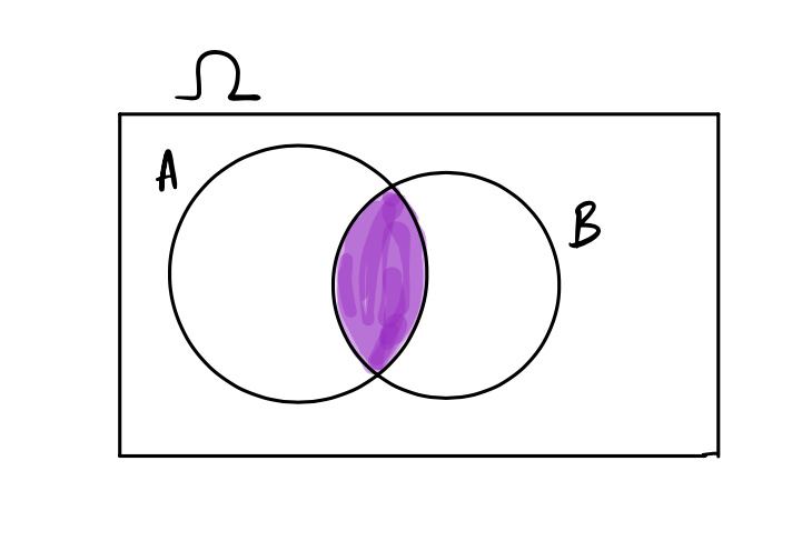
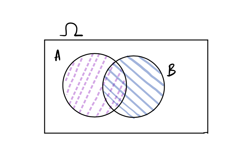
We often want to know the probability that two (or more) events will both happen: What is the probability if we roll a pair of dice, that both will show six spots; or if we deal two cards from a standard 52 card deck, that both would be kings, or in a family with two babies, both would suffer SIDS. What do we know? We can draw a Venn diagram to represent intersecting events:
This picture tells us that \(A\cap B\) (the purple shaded part, which represents the overlap: that is, the outcomes that are in both \(A\) and \(B\)) is inside both \(A\) and \(B\), so its probability should be less than each of \(P(A)\) and \(P(B)\): \(P(A\cap B) \le P(A), P(B)\). In fact, we write the probability of the intersection as:
\[P(A \cap B) = P(A) \times P(B|A)\] We read the second probability on the right-hand side of the equation as the conditional probability of \(B\) given \(A\). Note that \(B\vert A\) is not an event, but we use \(P(B\vert A)\) as a shorthand for the conditional probability of \(B\) given \(A\).
For example, in the example with the box with two red and two blue cards, let \(A\) be the event of drawing a red card on the first draw, and \(B\) be the event of drawing a blue card on the second draw. If we draw two cards without replacement, then we have that \(P(A) = \displaystyle \frac{2}{4}\), \(P(B | A) = \displaystyle \frac{2}{3}\) (the denominator reduces by one, since there are only 3 cards left in the box, of which 2 are blue). Therefore:
\[P(A \cap B) = P(A) \times P(B|A) = \frac{2}{4} \times \frac{2}{3} = \frac{1}{3}\] This becomes more clear if we think about the long run frequencies. We draw a red card first about half the time in the long run (if we repeated this experiment of drawing a card over and over again). Of those times, we would also draw a blue card second about two-thirds of the time, since drawing a blue card would be twice as likely as drawing a red card. Therefore drawing a red card first and then a blue card would happen two thirds of one half of the time, which is about a third of the time.
Note that the roles of \(A\) and \(B\) could be reversed in the expression above:
\[ P(A \cap B) = P(A) \times P(B | A) = P(B) \times P(A | B)\] This gives us a way to define the conditional probability, as long as we are not dividing by \(0\):
- Conditional probability of \(B\) given \(A\)
-
This is defined to be the probability of the intersection of \(A\) and \(B\), normalized by dividing by \(P(A)\):
\[ P(B | A) = \frac{ P(A \cap B)}{P(A)} \]
The idea here is that we know that \(A\) happened, therefore the only outcomes we are concerned about are the ones in \(A\) which has become our new outcome space, and we need to update the probability of \(B\). We can think about it as computing the “size” of the part of \(B\) that is possible, given the new information, that is,\(A\cap B\), relative to the size of the new outcome space (rather than relative to 1 which is the size of the original outcome space \(\Omega\). For example, our new probability of \(A\), denoted by \(P(A | A)\) will be 1!
Important caveats!!
\(P(B | A)\) denotes this new and updated probability, but \(B | A\) is not an event!
\(P(A | B)\) and \(P(B | A)\) can be very different!
Consider this scenario:
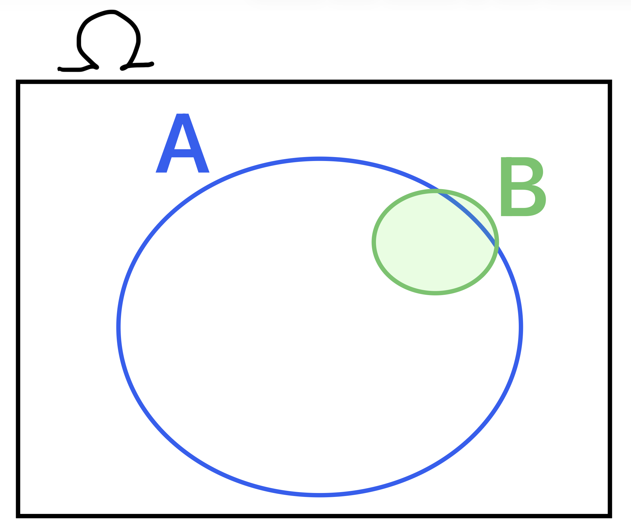
Note that B is almost entirely inside A.
Now what is \(P(A|B)\)? That is, given that B happened (we’re somewhere in the small circle), what’s the chance that A happened (we’re also in the big circle)?
Our formula says: \(P(A|B) = \frac{P(A \cap B)}{P(B)}\)
But look at the Venn diagram. Almost all of event B is also part of event A. If B happens, then A almost surely also happens. In other words, \(P(A \cap B) \approx P(B)\). Which means…
\(P(A|B) = \frac{P(A \cap B)}{P(B)} \approx \frac{P(B)}{P(B)} = 1\)
The opposite is not true, though.
\(P(B|A) = ?\)
Given that A happened (we’re somewhere in the big circle), what’s the chance that B happened (we’re also in the small circle)? Well, being in the big circle still doesn’t make B super likely, so \(P(B|A)\) is clearly much less than 100%.
\(P(B|A) = \frac{P(B \cap A)}{P(A)} \approx \frac{P(B)}{P(A)}\)
Which is much smaller than 1, because B is a lot smaller than A.
Independence
- Independent events
-
We say that two events are independent if the probabilities for the second event remain the same even if you know that the first event has happened, no matter how the first event turns out. Otherwise, the events are said to be dependent.
Example of independent events
Getting heads on one coin flip doesn’t change the chance of getting heads on a second coin flip. The flips are independent. Let’s name the events:
- Event \(A\) is “First coin flip is Heads.” \(P(A) = 0.5\)
- Event \(B\) is “Second coin flip is Heads.” \(P(B) = 0.5\)
If \(A\) happens (first flip is Heads), it doesn’t change \(P(B)\) (chance the second flip will be Heads). In other words:
\(P(B | A) = P(B) = 0.5\)
And if \(A\) doesn’t happen (\(A^C\), the first flip is Tails), this still doesn’t change \(P(B)\) (chance the second flip will be Heads).
\(P(B | A^C) = P(B) = 0.5\)
In other words, whatever happens with \(A\), the chance of \(B\) will not change. And vice versa.
Example of dependent events
Consider “sleeping through your alarm” to be an event, \(A\). Maybe you rarely do this, so \(P(A) = 0.02\). Now consider “being late to class” to be an event, \(B\). Maybe this is also uncommon for you, so \(P(B) = 0.10\). However, IF you missed your alarm, THEN you’re much more likely to be late for class! That is, given that you missed your alarm, you’re suddenly (say) 60% likely to be late. In other words,
- Event \(A\) is “Sleeping through your alarm.” \(P(A) = 0.02\)
- Event \(B\) is “Being late to class.” \(P(B) = 0.10\)
- \(P(B | A) = 0.60\) which is much bigger than \(P(B)\)
The events are dependent.
How to check for independence:
If \(A\) and \(B\) are independent, \(P(B|A) = P(B)\). (And \(P(A|B) = P(A)\))
Consequently, the multiplication rule reduces to:
\[ P(A \cap B) = P(A) \times P(B | A) = P(A) \times P(B) \]
Usually the fastest and most convenient way to check if two events are independent is to see if the product of their probabilities is the same as the probability of their intersection:
Computational check for independence
Check if: \(P(A \cap B) = P(A)\times P(B)\)
As another example, consider our box of 2 red and 2 blue tickets.
We’re going to draw twice from the box.
When we draw with replacement, the box resets to the same place between draws. If we get red ticket on the first draw, then put it back, the box is back to its original form: 2 red, 2 blue. This means the second draw faces the same probabilities as the first: the chance of the second ticket being red is still 1/2. Hence, the draws are independent.
However, if we draw the tickets without replacement, the box changes between draws, and so will the probabilities. If a red ticket comes out first, the box has only 1 red and 2 blue tickets left, so the probability of a red ticket on the second draw is now only 1/3. The draws are dependent.
The lesson here is that when we draw tickets with replacement, the draws are independent - the outcome of the first draw does not affect the second. If we draw tickets without replacement, the draws are dependent. The outcome of the first draw changes the probabilities of the tickets for the second draw.
Example: Selecting 2 people out of a group of 5
(drawing without replacement)
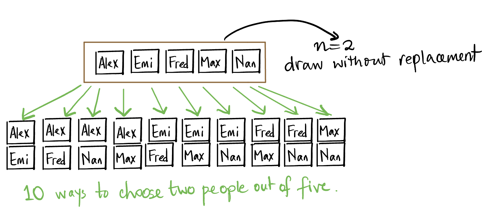
We have a group of 5 people: Alex, Emi, Fred, Max, and Nan. Two of the five are to be selected at random to form a two person committee. Represent this situation using draws from a box of tickets.
Check your answer
We only care about who is picked, not the order in which they are picked. For instance, picking Alex first and then Emi results in the same committee as picking Emi first and then Alex.
All the ten pairs are equally likely. On the first draw, there are 5 tickets to choose from, and on the second there are 4, making \(5 \times 4 = 20\) possible draws of two tickets, drawn from this box, one at a time, without replacement, but this counts drawing Alex first and then Emi as a different draw from Emi first and then Alex. However, since order does not matter when creating a committee, both these draws end up producing the same committee consisting of Emi and Alex. Therefore, there are 20 / 2 = 10 possible unique committees.
What is the probability that Alex and Emi will be selected? Guess! (Hint: you have seen all the possible pairs above, and they are equally likely. What will be the probability of any one of them?)
We could use the multiplication rule to compute this probability, which is much simpler than writing out all the possible outcomes. The committee can consist of Alex and Emi either if Alex is drawn first and Emi second, or Emi is drawn first and Alex second. The probability that Alex will be drawn first is \(1/5\). The conditional probability that Emi will be drawn second given that Alex was drawn is \(1/4\) since there are only 4 tickets left in the box. Using the multiplication rule, the probability that Alex will be drawn first and Emi second is \((1/4) \times (1/5) = 1/20\). Similarly, the probability that Emi will be drawn first and Alex second is \(1/20\). This means that the probability that Alex and Emi will be selected for the committee is \(1/20 + 1/20 = 1/10\).
Example: Colored and numbered tickets
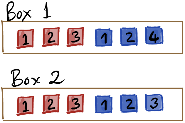
I have two boxes with numbered tickets colored red or blue as shown below.
Are color and number independent or dependent for box 1? What about box 2?
For example, is the probability of a ticket marked 1 the same whether the ticket is red or blue?
Check your answer
For box 1, color and number are dependent, since the probability of 3 given that the ticket is red is 1/3, but the probability of 3 given that the ticket is blue is 0 (and similarly for the probability of 4).
Even though the probability for 1 or 2 given the ticket is red is the same as the probability for 1 or 2 given the ticket is blue, we say that color and number are dependent because of the tickets marked 3 or 4.
Now you work it out for box 2.
Example: Tickets with more than one number on them
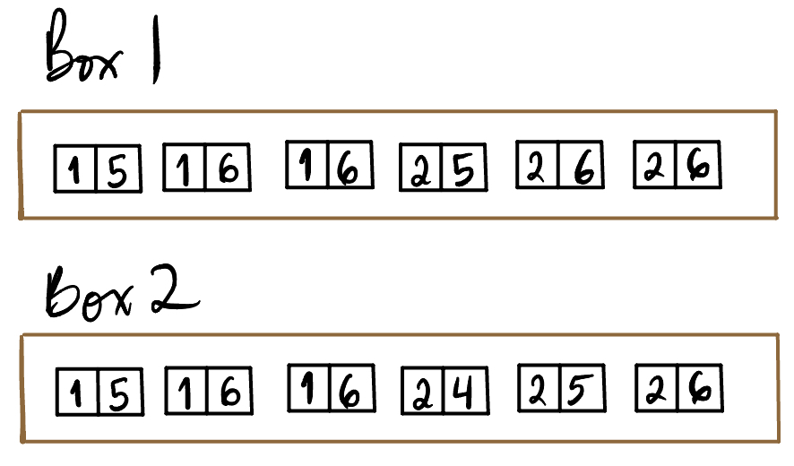
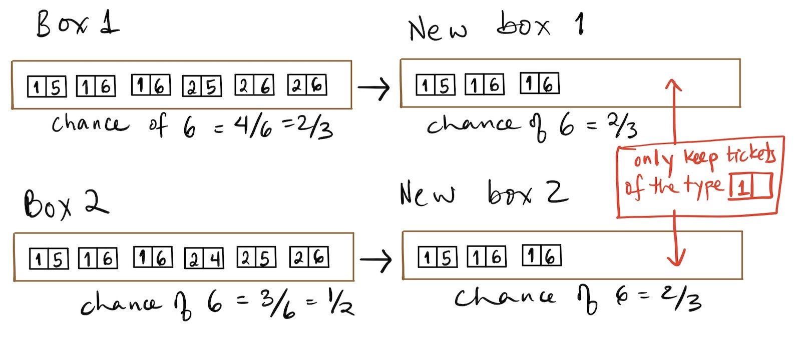
Now I have two boxes that with numbered tickets, where each ticket has two numbers on them, as shown. For each box, are the two numbers independent or dependent? For example, if I know that the first number is 1 does it change the probability of the second number being 6 (or the other way around: if I know the second number is 6, does it change the probability of the first number being 1)?
Check your answer
For box 1, the first number and second number are independent, as shown below, using 1 and 6 as examples. If we know that the first number is 1, the box reduces as shown. The probability of the second number being 6 does not change for box 1. The probability does change for box 2, increasing from 1/2 to 2/3, since the second number is more likely to be 6 if the first number is 1.
Back to Sally Clark
Professor Roy Meadow claimed that the probability of two of Sally Clark’s sons dying of SIDS was 1 in 73 million. He obtained this number by multiplying 8543 by 8543, using the multiplication rule, treating the two events as independent. The question is, are they really independent? Was a crime really committed? Unfortunately for Sally Clark, two catastrophic errors were committed in her case by the prosecution, and not caught by the defense. (She appealed the decision, and was acquitted and released, but after spending 4 years in prison after being accused of murdering her babies. You can imagine how she was treated.)
The first error was in treating the deaths as independent, and the second was in looking at the wrong probability. Let’s look at the first mistake. It turns out that the probability of a second child dying of “cot death” or SIDS is 1/60 given that the first child died of SIDS. This was a massive error, and it turned out that the prosecution suppressed the pathology reports for the second baby, who had a very bad infection and might have died of that. It is also believed that male infants are more likely to suffer cot death.
The second error is an example of what is called the Prosecutor’s Fallacy. What is needed is \(P(\text{innocence }\vert \text{ evidence})\), but it is often confused with (the much smaller) \(P(\text{evidence }\vert \text{ innocence})\). They should have actually compared the probability of innocence given the evidence with the probability of murder given the evidence. These multiple errors ruined many lives. Though Sally Clark was eventually acquitted, helped by the Royal Statistical Society’s evidence, her life was shattered, and she died soon after being released. The moral of this story is to be very careful while multiplying probabilities. You must check to see if the events are actually independent.
De Méré’s paradox
Let’s finally compute the probability of rolling at least one six in 4 rolls of a fair six-sided die. This is much easier to compute if we use the complement rule. The complement of at least one six is no sixes in 4 rolls. Each roll is independent of the other rolls because what you roll does not affect the values of future rolls. This means that we can use the multiplication rule to figure out the chance of no sixes in any of the rolls. The chance of no six in any particular roll is \(5/6\) (there are five outcomes that are not six).
The chance of no sixes in any of the 4 rolls is therefore \(\displaystyle \left( \frac{5}{6}\right)^4\) (because the rolls are independent). Using the complement rule, we get that: \[ P(\text{at least one six in 4 rolls}) = 1 - P(\text{no sixes in any of the 4 rolls}) = 1 - \left( \frac{5}{6}\right)^4 \approx 0.518\]
Similarly, the probability of at least 1 double six in 24 rolls of a pair of dice is given by \[ 1- P(\text{no double sixes in any of the 24 rolls}) = 1 - \left( \frac{35}{36}\right)^{24} \approx 0.491\]
By the way, notice that the simulation was pretty accurate!
Before we wrap up these notes, let’s review two important things. The first has to do with a very common misconception, confusing mutually exclusive and independent events.
Mutually exclusive vs independent events
Note that if two events \(A\) and \(B\), both with positive probability, are mutually exclusive, they cannot be independent. If \(P(A \cap B) = 0\), but neither \(P(A) =0\) nor \(P(B) = 0\), then \(P(A \cap B) = 0 \ne P(A)\times P(B)\). However, if two events are not independent, that does not mean they are mutually exclusive.
The second item generalizes the addition rule that we have already seen, by extending it to events that are not mutually exclusive. It is called the “inclusion-exclusion formula”.
Inclusion-exclusion (generalized addition rule)
Now that we know how to compute the probability of the intersection of two events, we can compute the probability of the union of two events:
\[P(A \cup B) = P(A) + P(B) - P(A \cap B) \]
You can see that if we just add the probabilities of \(A\) and \(B\), we double count the overlap. By subtracting it once, we can get the correct probability, and we know how to compute the probability of \(A\cap B\). This is known as the inclusion-exclusion principle.
Summary
In this lecture, we do a deep dive into computing probabilities. It is well known that people are just not good at estimating probabilities of events, and we saw the tragic example of Sally Clark (who, even more sadly, is not a unique case).
We defined conditional probability and independence, and the multiplication rule, considering draws at random with and without replacement. We finally computed the probabilities in the dice games from 17th century France by combining the multiplication rule and the complement rule.
We noted that independent events are very different from mutually exclusive events, and finally we learned how to compute probabilities of unions of events that may not be mutually exclusive with the inclusion-exclusion or generalized addition rule.