Extra Practice: Data Wrangling
Click to expand and work on the sections you need.
A good rule of thumb is this: do a bunch of problems in each section until you get bored because everything has gotten too easy.
Pipe Practice |>
From nested functions to pipelines and back again.
Write your code in the editor below each question, then click Run Code. The functions and datasets are already loaded for you.
In case you missed it, there’s a quick 12-second video demonstrating the pipe here.
Question 1: Square root of a mean
Rewrite these nested function calls as a single pipeline using |>.
numbers = c(4, 9, 16)

sqrt(mean(numbers))
Expected output is below, as a hint
[1] 3.109126Show answer
numbers |>
    mean() |>
    sqrt()
Note that whitespace is flexible - you can break a command into many lines (above) or put it all on one line (below). As long as a line is does not complete a command, R will keep reading, adding the next line to the current command. This is why we can break a pipeline into multiple lines IF we put the pipes at the end of lines, so the commands are left incomplete and R keeps reading.
For very short pipelines, one line will do. In most complex data-wrangling pipelines, where we often have longer lines of code, it is best to add a new line after every pipe operator |> to make the code easier to read.
numbers |> mean() |> sqrt()Question 2: Round a standard deviation
Rewrite the pipeline as nested function calls (without using |>).
numbers = c(2, 5, 8, 11)

numbers |>
    sd() |>
    round(digits = 2)
Expected output is below, as a hint
[1] 3.87Show answer
round(sd(numbers), digits = 2)Remember, the pipe just passes the thing to the left of the |> as the first argument to the function on the right. You can still put in second and third arguments etc as needed. So numbers |> sd() is equivalent to sd(numbers), and sd(numbers) |> round(digits = 2) is equivalent to round(sd(numbers), digits = 2).
Question 3: Endangered Species
Rewrite these nested function calls as a single pipeline using |>.
select(filter(msleep, conservation == "en"), name, sleep_total)Expected output is below, as a hint (first 4 rows)
# A tibble: 4 × 2
  name            sleep_total
  <chr>                 <dbl>
1 Asian elephant          3.9
2 Golden hamster         14.3
3 Tiger                  15.8
4 Giant armadillo        18.1
Show answer
msleep |>
    filter(conservation == "en") |>
    select(name, sleep_total)
Question 4: Sort the long sleepers
Rewrite this pipeline as nested function calls (without using |>).
msleep |>
    filter(sleep_total > 10) |>
    arrange(desc(sleep_total))
Expected output is below, as a hint (first 4 rows)
# A tibble: 44 × 11
  name                 genus      vore    order           conservation
  <chr>                <chr>      <chr>   <chr>           <chr>
1 Little brown bat     Myotis     insecti Chiroptera      <NA>
2 Big brown bat        Eptesicus  insecti Chiroptera      lc
3 Thick-tailed opposum Lutreolina carni   Didelphimorphia lc
4 Giant armadillo      Priodontes insecti Cingulata       en
  sleep_total sleep_rem sleep_cycle awake  brainwt bodywt
        <dbl>     <dbl>       <dbl> <dbl>    <dbl>  <dbl>
1        19.9       2         0.2     4.1  0.00025  0.01
2        19.7       3.9       0.117   4.3  0.0003   0.023
3        19.4       6.6      NA       4.6 NA        0.37
4        18.1       6.1      NA       5.9  0.081   60
# ℹ 40 more rows
Show answer
arrange(filter(msleep, sleep_total > 10), desc(sleep_total))Question 5: Sleep in minutes
Rewrite these nested function calls as a single pipeline using |>.
select(mutate(msleep, sleep_minutes = sleep_total * 60),
       name, sleep_minutes)
Expected output is below, as a hint (first 4 rows)
# A tibble: 83 × 2
  name                       sleep_minutes
  <chr>                              <dbl>
1 Cheetah                              726
2 Owl monkey                          1020
3 Mountain beaver                      864
4 Greater short-tailed shrew           894
# ℹ 79 more rows
Show answer
msleep |>
    mutate(sleep_minutes = sleep_total * 60) |>
    select(name, sleep_minutes)
Question 6: Average sleep by diet
Rewrite this pipeline as nested function calls (without using |>).
msleep |>
    group_by(vore) |>
    summarize(mean_sleep = mean(sleep_total))
Expected output is below, as a hint (first 4 rows)
# A tibble: 5 × 2
  vore    mean_sleep
  <chr>        <dbl>
1 carni        10.4
2 herbi         9.51
3 insecti      14.9
4 omni         10.9
# ℹ 1 more row
Show answer
summarize(group_by(msleep, vore),
          mean_sleep = mean(sleep_total))
Question 7: Average sleep of herbivores
Rewrite these nested function calls as a single pipeline using |>.
summarize(mutate(filter(msleep, vore == "herbi"),
                 sleep_minutes = sleep_total * 60),
          mean_minutes = mean(sleep_minutes))
Expected output is below, as a hint (first 1 row)
# A tibble: 1 × 1
  mean_minutes
         <dbl>
1         571.
Show answer
msleep |>
    filter(vore == "herbi") |>
    mutate(sleep_minutes = sleep_total * 60) |>
    summarize(mean_minutes = mean(sleep_minutes))
Question 8: Count animals by diet
Rewrite this pipeline as nested function calls (without using |>).
msleep |>
    group_by(vore) |>
    summarize(n = n()) |>
    arrange(desc(n))
Expected output is below, as a hint (first 4 rows)
# A tibble: 5 × 2
  vore      n
  <chr> <int>
1 herbi    32
2 omni     20
3 carni    19
4 <NA>      7
# ℹ 1 more row
Show answer
arrange(summarize(group_by(msleep, vore), n = n()),
        desc(n))
Question 9: Compare sleep variability
Rewrite these nested function calls as a single pipeline using |>.
arrange(summarize(group_by(filter(msleep, vore != "insecti"),
                           vore),
                  sd_sleep = sd(sleep_total)),
        desc(sd_sleep))
Expected output is below, as a hint (first 3 rows)
# A tibble: 3 × 2
  vore  sd_sleep
  <chr>    <dbl>
1 herbi     4.88
2 carni     4.67
3 omni      2.95
Show answer
msleep |>
    filter(vore != "insecti") |>
    group_by(vore) |>
    summarize(sd_sleep = sd(sleep_total)) |>
    arrange(desc(sd_sleep))
Question 10: Rank average body weights by diet
Rewrite this pipeline as nested function calls (without using |>).
msleep |>
    filter(sleep_total < 10) |>
    mutate(bodywt_g = bodywt * 1000) |>
    group_by(vore) |>
    summarize(mean_bodywt_g = mean(bodywt_g)) |>
    arrange(desc(mean_bodywt_g))
Expected output is below, as a hint (first 4 rows)
# A tibble: 5 × 2
  vore    mean_bodywt_g
  <chr>           <dbl>
1 herbi         733186.
2 carni         153029.
3 omni           22778.
4 insecti         2288.
# ℹ 1 more row
Show answer
arrange(summarize(group_by(mutate(filter(msleep, sleep_total < 10),
                                 bodywt_g = bodywt * 1000),
                          vore),
                  mean_bodywt_g = mean(bodywt_g)),
        desc(mean_bodywt_g))
Know when to use filter, select, mutate, summarize, arrange, and group_by
Fill in each blank with one function name: filter, select, mutate, summarize, arrange, or group_by. Replace the blank in each editor, then click Run Code. Each preview shows the first four rows and the columns relevant to the question; run the pipeline on the full msleep dataset.
Question 1: Weight in grams
Task: Add a bodywt_g column containing body weight in grams. The bodywt column is in kilograms. Keep all existing rows and columns.
Replace the blank with one of: filter, select, mutate, summarize, arrange, or group_by.
Preview of relevant columns of msleep:
| name | bodywt |
|---|---|
| Cheetah | 50.000 |
| Owl monkey | 0.480 |
| Mountain beaver | 1.350 |
| Greater short-tailed shrew | 0.019 |
Expected output is below, as a hint (first 4 rows)
# A tibble: 83 × 12
  name                       genus      vore  order        conservation
  <chr>                      <chr>      <chr> <chr>        <chr>
1 Cheetah                    Acinonyx   carni Carnivora    lc
2 Owl monkey                 Aotus      omni  Primates     <NA>
3 Mountain beaver            Aplodontia herbi Rodentia     nt
4 Greater short-tailed shrew Blarina    omni  Soricomorpha lc
  sleep_total sleep_rem sleep_cycle awake  brainwt bodywt bodywt_g
        <dbl>     <dbl>       <dbl> <dbl>    <dbl>  <dbl>    <dbl>
1        12.1      NA        NA      11.9 NA       50        50000
2        17         1.8      NA       7    0.0155   0.48       480
3        14.4       2.4      NA       9.6 NA        1.35      1350
4        14.9       2.3       0.133   9.1  0.00029  0.019       19
# ℹ 79 more rows
Show answer
Answer: mutate
msleep |>
    mutate(bodywt_g = bodywt * 1000)
Question 2: One overall average
Task: Return one row containing the mean daily sleep across all animals.
Replace the blank with one of: filter, select, mutate, summarize, arrange, or group_by.
Preview of relevant columns of msleep:
| name | sleep_total |
|---|---|
| Cheetah | 12.1 |
| Owl monkey | 17.0 |
| Mountain beaver | 14.4 |
| Greater short-tailed shrew | 14.9 |
Expected output is below, as a hint (first 1 row)
# A tibble: 1 × 1
  mean_sleep
       <dbl>
1       10.4
Show answer
Answer: summarize
msleep |>
    summarize(mean_sleep = mean(sleep_total))
Question 3: Small, long-sleeping animals
Task: Keep only animals that weigh less than 1 kilogram and sleep more than 12 hours per day.
Replace the blank with one of: filter, select, mutate, summarize, arrange, or group_by.
Preview of relevant columns of msleep:
| name | bodywt | sleep_total |
|---|---|---|
| Cheetah | 50.000 | 12.1 |
| Owl monkey | 0.480 | 17.0 |
| Mountain beaver | 1.350 | 14.4 |
| Greater short-tailed shrew | 0.019 | 14.9 |
Expected output is below, as a hint (first 4 rows)
# A tibble: 20 × 11
  name                       genus      vore    order        conservation
  <chr>                      <chr>      <chr>   <chr>        <chr>
1 Owl monkey                 Aotus      omni    Primates     <NA>
2 Greater short-tailed shrew Blarina    omni    Soricomorpha lc
3 Chinchilla                 Chinchilla herbi   Rodentia     domesticated
4 Big brown bat              Eptesicus  insecti Chiroptera   lc
  sleep_total sleep_rem sleep_cycle awake brainwt bodywt
        <dbl>     <dbl>       <dbl> <dbl>   <dbl>  <dbl>
1        17         1.8      NA       7   0.0155   0.48
2        14.9       2.3       0.133   9.1 0.00029  0.019
3        12.5       1.5       0.117  11.5 0.0064   0.42
4        19.7       3.9       0.117   4.3 0.0003   0.023
# ℹ 16 more rows
Show answer
Answer: filter
msleep |>
filter(bodywt < 1 & sleep_total > 12)filter is for rows, select is for columns
Question 4: Two diet categories
Task: Keep only animals whose diet is “carni” or “omni”.
Replace the blank with one of: filter, select, mutate, summarize, arrange, or group_by.
Preview of relevant columns of msleep:
| name | vore |
|---|---|
| Cheetah | carni |
| Owl monkey | omni |
| Mountain beaver | herbi |
| Greater short-tailed shrew | omni |
Expected output is below, as a hint (first 4 rows)
# A tibble: 39 × 11
  name                       genus       vore  order        conservation
  <chr>                      <chr>       <chr> <chr>        <chr>
1 Cheetah                    Acinonyx    carni Carnivora    lc
2 Owl monkey                 Aotus       omni  Primates     <NA>
3 Greater short-tailed shrew Blarina     omni  Soricomorpha lc
4 Northern fur seal          Callorhinus carni Carnivora    vu
  sleep_total sleep_rem sleep_cycle awake  brainwt bodywt
        <dbl>     <dbl>       <dbl> <dbl>    <dbl>  <dbl>
1        12.1      NA        NA      11.9 NA       50
2        17         1.8      NA       7    0.0155   0.48
3        14.9       2.3       0.133   9.1  0.00029  0.019
4         8.7       1.4       0.383  15.3 NA       20.5
# ℹ 35 more rows
Show answer
Answer: filter
msleep |>
filter(vore %in% c("carni", "omni"))filter is for rows, select is for columns
Question 5: Drop conservation status
Task: Remove the conservation column while keeping all other columns.
Replace the blank with one of: filter, select, mutate, summarize, arrange, or group_by.
Preview of relevant columns of msleep:
| name | vore | conservation |
|---|---|---|
| Cheetah | carni | lc |
| Owl monkey | omni | NA |
| Mountain beaver | herbi | nt |
| Greater short-tailed shrew | omni | lc |
Expected output is below, as a hint (first 4 rows)
# A tibble: 83 × 10
  name                       genus      vore  order        sleep_total sleep_rem
  <chr>                      <chr>      <chr> <chr>              <dbl>     <dbl>
1 Cheetah                    Acinonyx   carni Carnivora           12.1      NA
2 Owl monkey                 Aotus      omni  Primates            17         1.8
3 Mountain beaver            Aplodontia herbi Rodentia            14.4       2.4
4 Greater short-tailed shrew Blarina    omni  Soricomorpha        14.9       2.3
  sleep_cycle awake  brainwt bodywt
        <dbl> <dbl>    <dbl>  <dbl>
1      NA      11.9 NA       50
2      NA       7    0.0155   0.48
3      NA       9.6 NA        1.35
4       0.133   9.1  0.00029  0.019
# ℹ 79 more rows
Show answer
Answer: select
msleep |>
select(-conservation)filter is for rows, select is for columns
Question 6: Heaviest first
Task: Put the animals in order from greatest to least body weight.
Replace the blank with one of: filter, select, mutate, summarize, arrange, or group_by.
Preview of relevant columns of msleep:
| name | bodywt |
|---|---|
| Cheetah | 50.000 |
| Owl monkey | 0.480 |
| Mountain beaver | 1.350 |
| Greater short-tailed shrew | 0.019 |
Expected output is below, as a hint (first 4 rows)
# A tibble: 83 × 11
  name             genus         vore  order        conservation sleep_total
  <chr>            <chr>         <chr> <chr>        <chr>              <dbl>
1 African elephant Loxodonta     herbi Proboscidea  vu                   3.3
2 Asian elephant   Elephas       herbi Proboscidea  en                   3.9
3 Giraffe          Giraffa       herbi Artiodactyla cd                   1.9
4 Pilot whale      Globicephalus carni Cetacea      cd                   2.7
  sleep_rem sleep_cycle awake brainwt bodywt
      <dbl>       <dbl> <dbl>   <dbl>  <dbl>
1      NA            NA  20.7    5.71  6654
2      NA            NA  20.1    4.60  2547
3       0.4          NA  22.1   NA      900.
4       0.1          NA  21.4   NA      800
# ℹ 79 more rows
Show answer
Answer: arrange
msleep |>
    arrange(desc(bodywt))
Question 7: Names and diets
Task: Keep only the name and diet columns, in that order.
Replace the blank with one of: filter, select, mutate, summarize, arrange, or group_by.
Preview of relevant columns of msleep:
| name | vore | sleep_total |
|---|---|---|
| Cheetah | carni | 12.1 |
| Owl monkey | omni | 17.0 |
| Mountain beaver | herbi | 14.4 |
| Greater short-tailed shrew | omni | 14.9 |
Expected output is below, as a hint (first 4 rows)
# A tibble: 83 × 2
  name                       vore
  <chr>                      <chr>
1 Cheetah                    carni
2 Owl monkey                 omni
3 Mountain beaver            herbi
4 Greater short-tailed shrew omni
# ℹ 79 more rows
Show answer
Answer: select
msleep |>
select(name, vore)filter is for rows, select is for columns
Question 8: Count each animal order
Task: Count the animals separately for each taxonomic order.
Replace the blank with one of: filter, select, mutate, summarize, arrange, or group_by.
Preview of relevant columns of msleep:
| name | order |
|---|---|
| Cheetah | Carnivora |
| Owl monkey | Primates |
| Mountain beaver | Rodentia |
| Greater short-tailed shrew | Soricomorpha |
Expected output is below, as a hint (first 4 rows)
# A tibble: 19 × 2
  order        n_animals
  <chr>            <int>
1 Afrosoricida         1
2 Artiodactyla         6
3 Carnivora           12
4 Cetacea              3
# ℹ 15 more rows
Show answer
Answer: group_by
msleep |>
    group_by(order) |>
    summarize(n_animals = n())
Question 9: Only herbivores
Task: Keep only the herbivores, whose diet is recorded as “herbi”.
Replace the blank with one of: filter, select, mutate, summarize, arrange, or group_by.
Preview of relevant columns of msleep:
| name | vore |
|---|---|
| Cheetah | carni |
| Owl monkey | omni |
| Mountain beaver | herbi |
| Greater short-tailed shrew | omni |
Expected output is below, as a hint (first 4 rows)
# A tibble: 32 × 11
  name             genus      vore  order        conservation sleep_total
  <chr>            <chr>      <chr> <chr>        <chr>              <dbl>
1 Mountain beaver  Aplodontia herbi Rodentia     nt                  14.4
2 Cow              Bos        herbi Artiodactyla domesticated         4
3 Three-toed sloth Bradypus   herbi Pilosa       <NA>                14.4
4 Roe deer         Capreolus  herbi Artiodactyla lc                   3
  sleep_rem sleep_cycle awake brainwt bodywt
      <dbl>       <dbl> <dbl>   <dbl>  <dbl>
1       2.4      NA       9.6 NA        1.35
2       0.7       0.667  20    0.423  600
3       2.2       0.767   9.6 NA        3.85
4      NA        NA      21    0.0982  14.8
# ℹ 28 more rows
Show answer
Answer: filter
msleep |>
filter(vore == "herbi")filter is for rows, select is for columns
Question 10: Fraction of the day asleep
Task: Add a column containing the fraction of a 24-hour day each animal spends asleep. Keep all existing rows and columns.
Replace the blank with one of: filter, select, mutate, summarize, arrange, or group_by.
Preview of relevant columns of msleep:
| name | sleep_total |
|---|---|
| Cheetah | 12.1 |
| Owl monkey | 17.0 |
| Mountain beaver | 14.4 |
| Greater short-tailed shrew | 14.9 |
Expected output is below, as a hint (first 4 rows)
# A tibble: 83 × 12
  name                       genus      vore  order        conservation
  <chr>                      <chr>      <chr> <chr>        <chr>
1 Cheetah                    Acinonyx   carni Carnivora    lc
2 Owl monkey                 Aotus      omni  Primates     <NA>
3 Mountain beaver            Aplodontia herbi Rodentia     nt
4 Greater short-tailed shrew Blarina    omni  Soricomorpha lc
  sleep_total sleep_rem sleep_cycle awake  brainwt bodywt sleep_fraction
        <dbl>     <dbl>       <dbl> <dbl>    <dbl>  <dbl>          <dbl>
1        12.1      NA        NA      11.9 NA       50              0.504
2        17         1.8      NA       7    0.0155   0.48           0.708
3        14.4       2.4      NA       9.6 NA        1.35           0.6
4        14.9       2.3       0.133   9.1  0.00029  0.019          0.621
# ℹ 79 more rows
Show answer
Answer: mutate
msleep |>
    mutate(sleep_fraction = sleep_total / 24)
Question 11: Alphabetical carnivores
Task: Keep the carnivores (“carni”), then put their names in alphabetical order.
Replace the blank with one of: filter, select, mutate, summarize, arrange, or group_by.
Preview of relevant columns of msleep:
| name | vore |
|---|---|
| Cheetah | carni |
| Owl monkey | omni |
| Mountain beaver | herbi |
| Greater short-tailed shrew | omni |
Expected output is below, as a hint (first 4 rows)
# A tibble: 19 × 11
  name                 genus    vore  order     conservation sleep_total
  <chr>                <chr>    <chr> <chr>     <chr>              <dbl>
1 Arctic fox           Vulpes   carni Carnivora <NA>                12.5
2 Bottle-nosed dolphin Tursiops carni Cetacea   <NA>                 5.2
3 Caspian seal         Phoca    carni Carnivora vu                   3.5
4 Cheetah              Acinonyx carni Carnivora lc                  12.1
  sleep_rem sleep_cycle awake brainwt bodywt
      <dbl>       <dbl> <dbl>   <dbl>  <dbl>
1      NA            NA  11.5  0.0445   3.38
2      NA            NA  18.8 NA      173.
3       0.4          NA  20.5 NA       86
4      NA            NA  11.9 NA       50
# ℹ 15 more rows
Show answer
Answer: arrange
msleep |>
    filter(vore == "carni") |>
    arrange(name)
Question 12: Convert the existing sleep column
Task: Replace the values in sleep_total with minutes instead of hours, keeping all rows and other columns.
Replace the blank with one of: filter, select, mutate, summarize, arrange, or group_by.
Preview of relevant columns of msleep:
| name | sleep_total |
|---|---|
| Cheetah | 12.1 |
| Owl monkey | 17.0 |
| Mountain beaver | 14.4 |
| Greater short-tailed shrew | 14.9 |
Expected output is below, as a hint (first 4 rows)
# A tibble: 83 × 11
  name                       genus      vore  order        conservation
  <chr>                      <chr>      <chr> <chr>        <chr>
1 Cheetah                    Acinonyx   carni Carnivora    lc
2 Owl monkey                 Aotus      omni  Primates     <NA>
3 Mountain beaver            Aplodontia herbi Rodentia     nt
4 Greater short-tailed shrew Blarina    omni  Soricomorpha lc
  sleep_total sleep_rem sleep_cycle awake  brainwt bodywt
        <dbl>     <dbl>       <dbl> <dbl>    <dbl>  <dbl>
1         726      NA        NA      11.9 NA       50
2        1020       1.8      NA       7    0.0155   0.48
3         864       2.4      NA       9.6 NA        1.35
4         894       2.3       0.133   9.1  0.00029  0.019
# ℹ 79 more rows
Show answer
Answer: mutate
msleep |>
    mutate(sleep_total = sleep_total * 60)
Question 13: Count each diet
Task: Return one row per diet category, with the number of animals in that category.
Replace the blank with one of: filter, select, mutate, summarize, arrange, or group_by.
Preview of relevant columns of msleep:
| name | vore |
|---|---|
| Cheetah | carni |
| Owl monkey | omni |
| Mountain beaver | herbi |
| Greater short-tailed shrew | omni |
Expected output is below, as a hint (first 4 rows)
# A tibble: 5 × 2
  vore    n_animals
  <chr>       <int>
1 carni          19
2 herbi          32
3 insecti         5
4 omni           20
# ℹ 1 more row
Show answer
Answer: summarize
msleep |>
    group_by(vore) |>
    summarize(n_animals = n())
Question 14: Shortest sleepers first
Task: Put the animals in order from least to most daily sleep.
Replace the blank with one of: filter, select, mutate, summarize, arrange, or group_by.
Preview of relevant columns of msleep:
| name | sleep_total |
|---|---|
| Cheetah | 12.1 |
| Owl monkey | 17.0 |
| Mountain beaver | 14.4 |
| Greater short-tailed shrew | 14.9 |
Expected output is below, as a hint (first 4 rows)
# A tibble: 83 × 11
  name        genus         vore  order          conservation sleep_total
  <chr>       <chr>         <chr> <chr>          <chr>              <dbl>
1 Giraffe     Giraffa       herbi Artiodactyla   cd                   1.9
2 Pilot whale Globicephalus carni Cetacea        cd                   2.7
3 Horse       Equus         herbi Perissodactyla domesticated         2.9
4 Roe deer    Capreolus     herbi Artiodactyla   lc                   3
  sleep_rem sleep_cycle awake brainwt bodywt
      <dbl>       <dbl> <dbl>   <dbl>  <dbl>
1       0.4          NA  22.1 NA       900.
2       0.1          NA  21.4 NA       800
3       0.6           1  21.1  0.655   521
4      NA            NA  21    0.0982   14.8
# ℹ 79 more rows
Show answer
Answer: arrange
msleep |>
    arrange(sleep_total)
Question 15: Sleep by conservation status
Task: Calculate a separate mean daily sleep for each conservation status.
Replace the blank with one of: filter, select, mutate, summarize, arrange, or group_by.
Preview of relevant columns of msleep:
| name | conservation | sleep_total |
|---|---|---|
| Cheetah | lc | 12.1 |
| Owl monkey | NA | 17.0 |
| Mountain beaver | nt | 14.4 |
| Greater short-tailed shrew | lc | 14.9 |
Expected output is below, as a hint (first 4 rows)
# A tibble: 7 × 2
  conservation mean_sleep
  <chr>             <dbl>
1 cd                 2.3
2 domesticated       7.58
3 en                13.0
4 lc                11.4
# ℹ 3 more rows
Show answer
Answer: group_by
msleep |>
    group_by(conservation) |>
    summarize(mean_sleep = mean(sleep_total))
Question 16: The longest sleep duration
Task: Return one row containing the largest daily sleep duration in the dataset.
Replace the blank with one of: filter, select, mutate, summarize, arrange, or group_by.
Preview of relevant columns of msleep:
| name | sleep_total |
|---|---|
| Cheetah | 12.1 |
| Owl monkey | 17.0 |
| Mountain beaver | 14.4 |
| Greater short-tailed shrew | 14.9 |
Expected output is below, as a hint (first 1 row)
# A tibble: 1 × 1
  max_sleep
      <dbl>
1      19.9
Show answer
Answer: summarize
msleep |>
    summarize(max_sleep = max(sleep_total))
Question 17: Long sleepers
Task: Keep only animals that sleep more than 10 hours per day.
Replace the blank with one of: filter, select, mutate, summarize, arrange, or group_by.
Preview of relevant columns of msleep:
| name | sleep_total |
|---|---|
| Cheetah | 12.1 |
| Owl monkey | 17.0 |
| Mountain beaver | 14.4 |
| Greater short-tailed shrew | 14.9 |
Expected output is below, as a hint (first 4 rows)
# A tibble: 44 × 11
  name                       genus      vore  order        conservation
  <chr>                      <chr>      <chr> <chr>        <chr>
1 Cheetah                    Acinonyx   carni Carnivora    lc
2 Owl monkey                 Aotus      omni  Primates     <NA>
3 Mountain beaver            Aplodontia herbi Rodentia     nt
4 Greater short-tailed shrew Blarina    omni  Soricomorpha lc
  sleep_total sleep_rem sleep_cycle awake  brainwt bodywt
        <dbl>     <dbl>       <dbl> <dbl>    <dbl>  <dbl>
1        12.1      NA        NA      11.9 NA       50
2        17         1.8      NA       7    0.0155   0.48
3        14.4       2.4      NA       9.6 NA        1.35
4        14.9       2.3       0.133   9.1  0.00029  0.019
# ℹ 40 more rows
Show answer
Answer: filter
msleep |>
filter(sleep_total > 10)filter is for rows, select is for columns
Question 18: Average sleep for each diet
Task: Calculate a separate mean daily sleep for each diet category.
Replace the blank with one of: filter, select, mutate, summarize, arrange, or group_by.
Preview of relevant columns of msleep:
| name | vore | sleep_total |
|---|---|---|
| Cheetah | carni | 12.1 |
| Owl monkey | omni | 17.0 |
| Mountain beaver | herbi | 14.4 |
| Greater short-tailed shrew | omni | 14.9 |
Expected output is below, as a hint (first 4 rows)
# A tibble: 5 × 2
  vore    mean_sleep
  <chr>        <dbl>
1 carni        10.4
2 herbi         9.51
3 insecti      14.9
4 omni         10.9
# ℹ 1 more row
Show answer
Answer: group_by
msleep |>
    group_by(vore) |>
    summarize(mean_sleep = mean(sleep_total))
Question 19: Keep two columns after filtering
Task: Among animals sleeping more than 10 hours per day, keep only name and sleep_total.
Replace the blank with one of: filter, select, mutate, summarize, arrange, or group_by.
Preview of relevant columns of msleep:
| name | vore | sleep_total |
|---|---|---|
| Cheetah | carni | 12.1 |
| Owl monkey | omni | 17.0 |
| Mountain beaver | herbi | 14.4 |
| Greater short-tailed shrew | omni | 14.9 |
Expected output is below, as a hint (first 4 rows)
# A tibble: 44 × 2
  name                       sleep_total
  <chr>                            <dbl>
1 Cheetah                           12.1
2 Owl monkey                        17
3 Mountain beaver                   14.4
4 Greater short-tailed shrew        14.9
# ℹ 40 more rows
Show answer
Answer: select
msleep |>
    filter(sleep_total > 10) |>
select(name, sleep_total)filter is for rows, select is for columns
Question 20: Sleep in minutes
Task: Add a column giving daily sleep in minutes. Keep all existing rows and columns.
Replace the blank with one of: filter, select, mutate, summarize, arrange, or group_by.
Preview of relevant columns of msleep:
| name | sleep_total |
|---|---|
| Cheetah | 12.1 |
| Owl monkey | 17.0 |
| Mountain beaver | 14.4 |
| Greater short-tailed shrew | 14.9 |
Expected output is below, as a hint (first 4 rows)
# A tibble: 83 × 12
  name                       genus      vore  order        conservation
  <chr>                      <chr>      <chr> <chr>        <chr>
1 Cheetah                    Acinonyx   carni Carnivora    lc
2 Owl monkey                 Aotus      omni  Primates     <NA>
3 Mountain beaver            Aplodontia herbi Rodentia     nt
4 Greater short-tailed shrew Blarina    omni  Soricomorpha lc
  sleep_total sleep_rem sleep_cycle awake  brainwt bodywt sleep_minutes
        <dbl>     <dbl>       <dbl> <dbl>    <dbl>  <dbl>         <dbl>
1        12.1      NA        NA      11.9 NA       50               726
2        17         1.8      NA       7    0.0155   0.48           1020
3        14.4       2.4      NA       9.6 NA        1.35            864
4        14.9       2.3       0.133   9.1  0.00029  0.019           894
# ℹ 79 more rows
Show answer
Answer: mutate
msleep |>
    mutate(sleep_minutes = sleep_total * 60)
Practice with conditions for filtering == != > >= < <= %in% & |
Use diamonds, a dataset of 53,940 diamonds included in ggplot2. Each row is one diamond. price is in US dollars, carat measures weight, and x y and z measure the length width and height of the diamond, in millimeters. cut, color, and clarity are other meaningful attributes that diamond-appraisers consider.
For each question, you’ll replace the blank inside filter() with one or more conditions, then click Run Code. Keep all columns. The dataset is already loaded.
Preview of diamonds (first 4 rows, all 10 columns):
| carat | cut | color | clarity | depth | table | price | x | y | z |
|---|---|---|---|---|---|---|---|---|---|
| 0.23 | Ideal | E | SI2 | 61.5 | 55 | 326 | 3.95 | 3.98 | 2.43 |
| 0.21 | Premium | E | SI1 | 59.8 | 61 | 326 | 3.89 | 3.84 | 2.31 |
| 0.23 | Good | E | VS1 | 56.9 | 65 | 327 | 4.05 | 4.07 | 2.31 |
| 0.29 | Premium | I | VS2 | 62.4 | 58 | 334 | 4.20 | 4.23 | 2.63 |
Question 1: A price ceiling
Task: Keep diamonds that cost at most $800.
Replace the blank inside filter() with the condition(s) that select these diamonds.
Expected output is below, as a hint (first 4 rows)
# A tibble: 9,804 × 10
  carat cut     color clarity depth table price     x     y     z
  <dbl> <ord>   <ord> <ord>   <dbl> <dbl> <int> <dbl> <dbl> <dbl>
1  0.23 Ideal   E     SI2      61.5    55   326  3.95  3.98  2.43
2  0.21 Premium E     SI1      59.8    61   326  3.89  3.84  2.31
3  0.23 Good    E     VS1      56.9    65   327  4.05  4.07  2.31
4  0.29 Premium I     VS2      62.4    58   334  4.2   4.23  2.63
# ℹ 9,800 more rows
Show answer
diamonds |>
    filter(price <= 800)
Question 2: Skip one cut
Task: Keep diamonds whose cut is not “Premium”.
Replace the blank inside filter() with the condition(s) that select these diamonds.
Expected output is below, as a hint (first 4 rows)
# A tibble: 40,149 × 10
  carat cut       color clarity depth table price     x     y     z
  <dbl> <ord>     <ord> <ord>   <dbl> <dbl> <int> <dbl> <dbl> <dbl>
1  0.23 Ideal     E     SI2      61.5    55   326  3.95  3.98  2.43
2  0.23 Good      E     VS1      56.9    65   327  4.05  4.07  2.31
3  0.31 Good      J     SI2      63.3    58   335  4.34  4.35  2.75
4  0.24 Very Good J     VVS2     62.8    57   336  3.94  3.96  2.48
# ℹ 40,145 more rows
Show answer
diamonds |>
    filter(cut != "Premium")
Question 3: More than one carat
Task: Keep diamonds weighing more than 1 carat.
Replace the blank inside filter() with the condition(s) that select these diamonds.
Expected output is below, as a hint (first 4 rows)
# A tibble: 17,502 × 10
  carat cut       color clarity depth table price     x     y     z
  <dbl> <ord>     <ord> <ord>   <dbl> <dbl> <int> <dbl> <dbl> <dbl>
1  1.17 Very Good J     I1       60.2    61  2774  6.83  6.9   4.13
2  1.01 Premium   F     I1       61.8    60  2781  6.39  6.36  3.94
3  1.01 Fair      E     I1       64.5    58  2788  6.29  6.21  4.03
4  1.01 Premium   H     SI2      62.7    59  2788  6.31  6.22  3.93
# ℹ 17,498 more rows
Show answer
diamonds |>
    filter(carat > 1)
Question 4: One clarity grade
Task: Keep diamonds whose clarity is “VS2”.
Replace the blank inside filter() with the condition(s) that select these diamonds.
Expected output is below, as a hint (first 4 rows)
# A tibble: 12,258 × 10
  carat cut       color clarity depth table price     x     y     z
  <dbl> <ord>     <ord> <ord>   <dbl> <dbl> <int> <dbl> <dbl> <dbl>
1  0.29 Premium   I     VS2      62.4    58   334  4.2   4.23  2.63
2  0.22 Fair      E     VS2      65.1    61   337  3.87  3.78  2.49
3  0.23 Very Good E     VS2      63.8    55   352  3.85  3.92  2.48
4  0.3  Very Good J     VS2      62.2    57   357  4.28  4.3   2.67
# ℹ 12,254 more rows
Show answer
diamonds |>
    filter(clarity == "VS2")
Question 5: At least five millimeters
Task: Keep diamonds whose length (x)is at least 5 mm.
Replace the blank inside filter() with the condition(s) that select these diamonds.
Expected output is below, as a hint (first 4 rows)
# A tibble: 36,354 × 10
  carat cut       color clarity depth table price     x     y     z
  <dbl> <ord>     <ord> <ord>   <dbl> <dbl> <int> <dbl> <dbl> <dbl>
1  0.7  Ideal     E     SI1      62.5    57  2757  5.7   5.72  3.57
2  0.86 Fair      E     SI2      55.1    69  2757  6.45  6.33  3.52
3  0.7  Ideal     G     VS2      61.6    56  2757  5.7   5.67  3.5
4  0.71 Very Good E     VS2      62.4    57  2759  5.68  5.73  3.56
# ℹ 36,350 more rows
Show answer
diamonds |>
    filter(x >= 5)
Question 6: Below half a carat
Task: Keep diamonds weighing less than 0.5 carats.
Replace the blank inside filter() with the condition(s) that select these diamonds.
Expected output is below, as a hint (first 4 rows)
# A tibble: 17,674 × 10
  carat cut     color clarity depth table price     x     y     z
  <dbl> <ord>   <ord> <ord>   <dbl> <dbl> <int> <dbl> <dbl> <dbl>
1  0.23 Ideal   E     SI2      61.5    55   326  3.95  3.98  2.43
2  0.21 Premium E     SI1      59.8    61   326  3.89  3.84  2.31
3  0.23 Good    E     VS1      56.9    65   327  4.05  4.07  2.31
4  0.29 Premium I     VS2      62.4    58   334  4.2   4.23  2.63
# ℹ 17,670 more rows
Show answer
diamonds |>
    filter(carat < 0.5)
Question 7: Large or inexpensive
Task: Keep diamonds that weigh at least 2 carats or cost less than $500 (or both).
Replace the blank inside filter() with the condition(s) that select these diamonds.
Expected output is below, as a hint (first 4 rows)
# A tibble: 3,883 × 10
  carat cut     color clarity depth table price     x     y     z
  <dbl> <ord>   <ord> <ord>   <dbl> <dbl> <int> <dbl> <dbl> <dbl>
1  0.23 Ideal   E     SI2      61.5    55   326  3.95  3.98  2.43
2  0.21 Premium E     SI1      59.8    61   326  3.89  3.84  2.31
3  0.23 Good    E     VS1      56.9    65   327  4.05  4.07  2.31
4  0.29 Premium I     VS2      62.4    58   334  4.2   4.23  2.63
# ℹ 3,879 more rows
Show answer
diamonds |>
    filter(carat >= 2 | price < 500)
Question 8: Two cuts within budget
Task: Keep diamonds whose cut is either “Ideal” or “Premium” and whose price is at most $1,500. Use %in% to specify the two cuts.
Replace the blank inside filter() with the condition(s) that select these diamonds.
Expected output is below, as a hint (first 4 rows)
# A tibble: 14,010 × 10
  carat cut     color clarity depth table price     x     y     z
  <dbl> <ord>   <ord> <ord>   <dbl> <dbl> <int> <dbl> <dbl> <dbl>
1  0.23 Ideal   E     SI2      61.5    55   326  3.95  3.98  2.43
2  0.21 Premium E     SI1      59.8    61   326  3.89  3.84  2.31
3  0.29 Premium I     VS2      62.4    58   334  4.2   4.23  2.63
4  0.23 Ideal   J     VS1      62.8    56   340  3.93  3.9   2.46
# ℹ 14,006 more rows
Show answer
diamonds |>
    filter(cut %in% c("Ideal", "Premium") & price <= 1500)
Question 9: Either cut, with a price limit
Task: Keep diamonds whose cut is “Fair” or “Good”, with a price below $1,000 in either case. Use both | and & in your condition.
Replace the blank inside filter() with the condition(s) that select these diamonds.
Expected output is below, as a hint (first 4 rows)
# A tibble: 1,221 × 10
  carat cut   color clarity depth table price     x     y     z
  <dbl> <ord> <ord> <ord>   <dbl> <dbl> <int> <dbl> <dbl> <dbl>
1  0.23 Good  E     VS1      56.9    65   327  4.05  4.07  2.31
2  0.31 Good  J     SI2      63.3    58   335  4.34  4.35  2.75
3  0.22 Fair  E     VS2      65.1    61   337  3.87  3.78  2.49
4  0.3  Good  J     SI1      64      55   339  4.25  4.28  2.73
# ℹ 1,217 more rows
Show answer
diamonds |>
    filter((cut == "Fair" | cut == "Good") & price < 1000)
Question 10: Exclude three colors
Task: Keep diamonds weighing more than 1 carat whose color is not “D”, “E”, or “F”. Use ! and %in% to exclude those colors. This one is tricky, you may have to tinker with the syntaxa bit to find what works.
Replace the blank inside filter() with the condition(s) that select these diamonds.
Expected output is below, as a hint (first 4 rows)
# A tibble: 11,688 × 10
  carat cut       color clarity depth table price     x     y     z
  <dbl> <ord>     <ord> <ord>   <dbl> <dbl> <int> <dbl> <dbl> <dbl>
1  1.17 Very Good J     I1       60.2    61  2774  6.83  6.9   4.13
2  1.01 Premium   H     SI2      62.7    59  2788  6.31  6.22  3.93
3  1.05 Very Good J     SI2      63.2    56  2789  6.49  6.45  4.09
4  1.05 Fair      J     SI2      65.8    59  2789  6.41  6.27  4.18
# ℹ 11,684 more rows
Show answer
diamonds |>
filter(carat > 1 & !(color %in% c("D", "E", "F")))Real tasks: I give you a problem, you build the pipeline
Each problem below should be answered with one single pipeline. Each problem uses a different dataset that is already loaded for you (they are all from tidyverse).
Question 1: mpg - car fuel efficiency data
The mpg dataset records fuel economy for different car models and configurations. cty and hwy are city and highway fuel economy in miles per gallon; higher values mean greater fuel efficiency. cyl is the number of “cylinders” (pistons) in the engine, and class is a broad category of vehicle type.
Preview of relevant columns of mpg (first 4 rows):
| manufacturer | model | year | cyl | cty | hwy | class |
|---|---|---|---|---|---|---|
| audi | a4 | 1999 | 4 | 18 | 29 | compact |
| audi | a4 | 1999 | 4 | 21 | 29 | compact |
| audi | a4 | 2008 | 4 | 20 | 31 | compact |
| audi | a4 | 2008 | 4 | 21 | 30 | compact |
Task: In one pipeline, make a shortlist of fuel-efficient cars. Keep cars with highway fuel economy of at least 30 miles per gallon, and return only manufacturer, model, cty, and hwy columns, in that order. Sort them from most to least fuel efficient in highway driving.
Expected output is below, as a hint (first 4 rows)
# A tibble: 26 × 4
  manufacturer model        cty   hwy
  <chr>        <chr>      <int> <int>
1 volkswagen   jetta         33    44
2 volkswagen   new beetle    35    44
3 volkswagen   new beetle    29    41
4 toyota       corolla       28    37
# ℹ 22 more rows
Show answer
mpg |>
    filter(hwy >= 30) |>
    select(manufacturer, model, cty, hwy) |>
    arrange(desc(hwy))
Note: A model can appear more than once because the data include different configurations of the same car.
Question 2: starwars - Star Wars characters
The starwars dataset has one row per character in the Star Wars film series. The characters in these films include humans among many other types of beings. species identifies the character’s species, height is in centimeters, mass is in kilograms. Some values may be missing (NA).
Here are a few rows of starwars:
| name | species | height | mass |
|---|---|---|---|
| Chewbacca | Wookiee | 228 | 112 |
| Roos Tarpals | Gungan | 224 | 82 |
| Poe Dameron | Human | NA | NA |
| BB8 | Droid | NA | NA |
| Bib Fortuna | Twi’lek | 180 | NA |
| R5-D4 | Droid | 97 | 32 |
| Tarfful | Wookiee | 234 | 136 |
| Ayla Secura | Twi’lek | 178 | 55 |
| Jar Jar Binks | Gungan | 196 | 66 |
| Jango Fett | Human | 183 | 79 |
Task: How do the heights and weights of Humans, Droids, and Wookiees compare? These are three of the species types in the Star Wars universe. We aren’t concerned with any other species. Write a single pipeline that produces a table with the average height, average mass, and total number of characters in each of these three species. Hint: use na.rm = TRUE when computing means.
Expected output is below, as a hint (first 3 rows)
# A tibble: 3 × 4
  species mean_height_cm mean_mass_kg n_characters
  <chr>            <dbl>        <dbl>        <int>
1 Droid             131.         69.8            6
2 Human             178          81.3           35
3 Wookiee           231         124              2
Show answer
starwars |>
    filter(species %in% c("Human", "Droid", "Wookiee")) |>
    group_by(species) |>
    summarize(mean_height_cm = mean(height, na.rm = TRUE),
              mean_mass_kg = mean(mass, na.rm = TRUE),
              n_characters = n())
Note: n_characters includes characters with missing height or weight data, while the means of height and weight use only characters with known measurements.
Question 3: economics - US economic measurements
The economics dataset contains yearly US economic measurements. Each row is one complete calendar year. year is an ordinary number, and unemploy is the average monthly number of unemployed people during that year, in thousands. This prepared dataset is already loaded.
Preview of relevant columns of economics (first 4 rows):
| year | unemploy |
|---|---|
| 1968 | 2797.417 |
| 1969 | 2830.167 |
| 1970 | 4127.333 |
| 1971 | 5021.667 |
Task: Make line plot of the number of unemployed people in millions over time, starting in the year 2000. Give the axes readable labels.
Expected output is below, as a hint
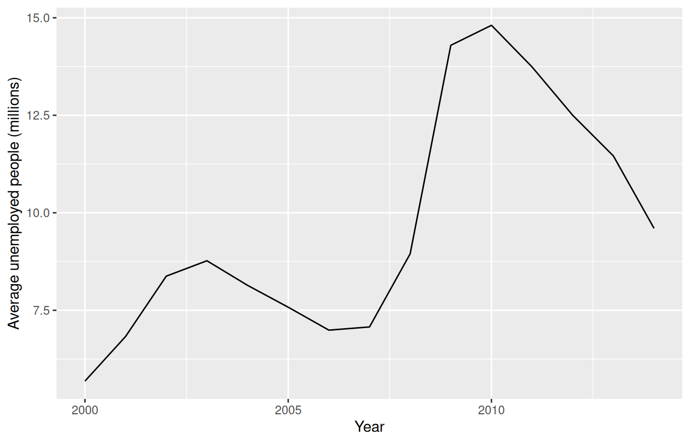
Show answer
economics |>
    filter(year >= 2000) |>
    mutate(unemployed_millions = unemploy / 1000) |>
    ggplot(aes(x = year, y = unemployed_millions)) +
    geom_line() +
    labs(x = "Year", y = "Average unemployed people (millions)")
Question 4: midwest - US county demographics in the Midwest states
The midwest dataset has one row per county (a county is a subdivision of a state). state is the state abbreviation (e.g., “OH” for Ohio), inmetro is 1 for metropolitan counties and 0 otherwise, poptotal is the population, and percbelowpoverty is the percentage of people below the poverty line.
Preview of relevant columns of midwest (first 4 rows):
| county | state | inmetro | poptotal | percbelowpoverty |
|---|---|---|---|---|
| ADAMS | IL | 0 | 66090 | 13.151443 |
| ALEXANDER | IL | 0 | 10626 | 32.244278 |
| BOND | IL | 0 | 14991 | 12.068844 |
| BOONE | IL | 1 | 30806 | 7.209019 |
Task: Calculate the total number of counties, total population, and average county poverty rate for only metropolitan counties each state. This last quantity should give every county equal weight, which is not exactly correct approach but fine for this exercise.
Expected output is below, as a hint (first 4 rows)
# A tibble: 5 × 4
  state n_counties total_pop_millions mean_county_poverty_pct
  <chr>      <int>              <dbl>                   <dbl>
1 IL            28               9.57                    9.56
2 IN            37               3.96                    9.59
3 MI            25               7.70                   11.3
4 OH            40               8.91                   11.5
# ℹ 1 more row
Show answer
midwest |>
    filter(inmetro == 1) |>
    mutate(pop_millions = poptotal / 1000000) |>
    group_by(state) |>
    summarize(n_counties = n(),
              total_pop_millions = sum(pop_millions),
              mean_county_poverty_pct = mean(percbelowpoverty))
Question 5: txhousing - Texas housing data
For this exercise, txhousing contains data on median home price sales in cities in Texas over various years. median_price is the median home sale price in dollars that year.
Preview of relevant columns of txhousing (first 4 rows):
| city | year | median_price |
|---|---|---|
| Abilene | 2000 | 71400 |
| Abilene | 2001 | 64500 |
| Abilene | 2002 | 64000 |
| Abilene | 2003 | 70000 |
Task: How do home prices in “Austin”, “Dallas”, and “Houston” compare over time? Make a plot of the median sale prices in thousands of dollars for these three cities over the years. Use a separate colored line for each city. Create readable axis labels and add a sensible title.
Expected output is below, as a hint
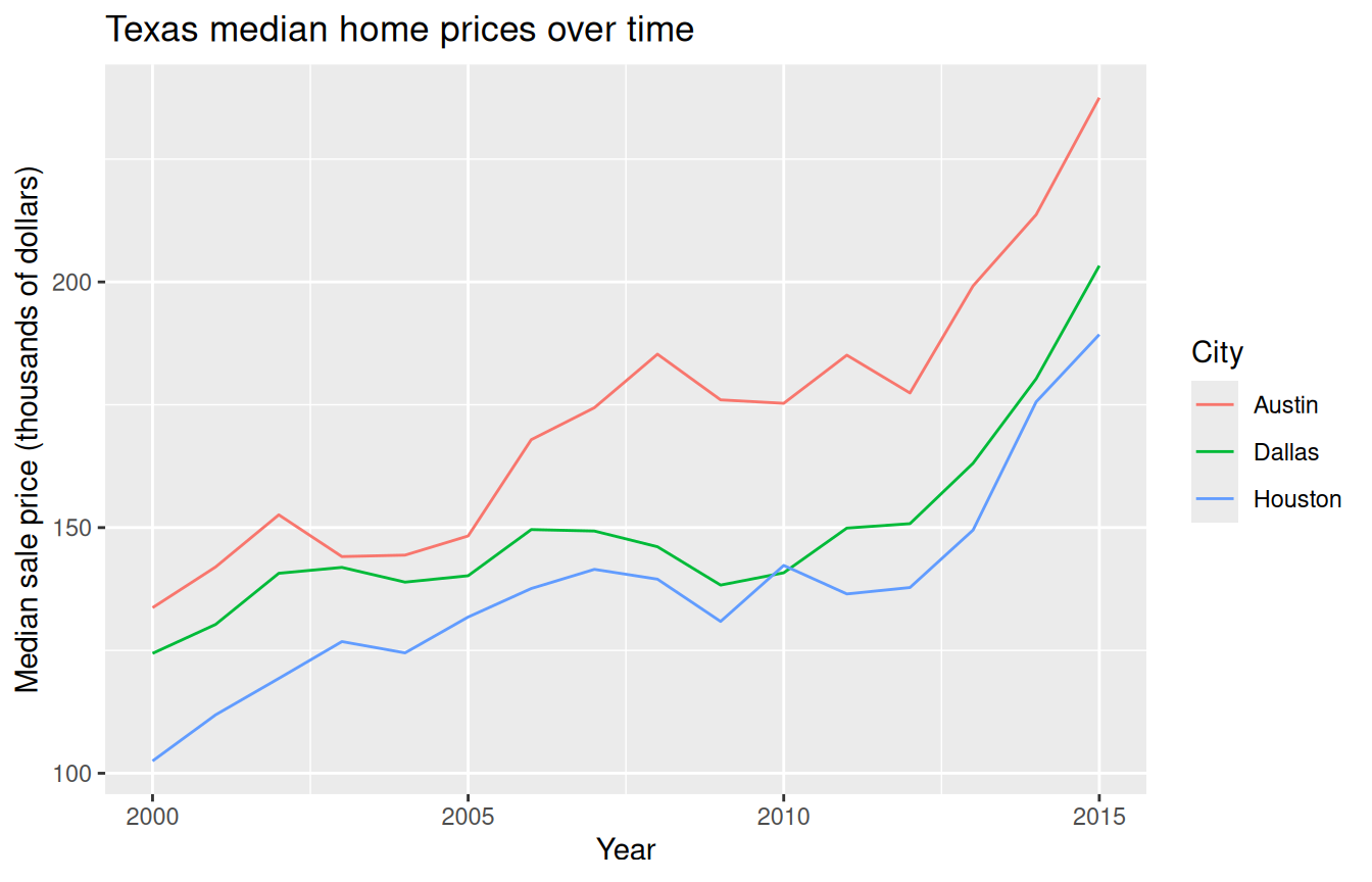
Show answer
txhousing |>
    filter(city %in% c("Austin", "Dallas", "Houston")) |>
    mutate(median_thousands = median_price / 1000) |>
    ggplot(aes(x = year, y = median_thousands, color = city)) +
    geom_line() +
    labs(x = "Year", y = "Median sale price (thousands of dollars)",
         color = "City",
         title = "Texas median home prices over time")
You can also do quick calculations directly in ggplot to save yourself a step:
txhousing |>
    filter(city %in% c("Austin", "Dallas", "Houston")) |>
    ggplot(aes(x = year, y = median_price / 1000, color = city)) +
    geom_line() +
    labs(x = "Year", y = "Median sale price (thousands of dollars)",
         color = "City",
         title = "Texas median home prices over time")