Hypothesis Tests II

STAT 20: Introduction to Probability and Statistics

Agenda

• Announcements
• Reading Questions: Hypothesis Tests II
• Break
• Worksheet: Hypothesis Tests II
• Appendix

Announcements

• Quiz 3 on Thursday

• Portfolio 5 (Mon., Tue., Wed.) due Friday at 5pm

Reading Questions

• Please put your laptops under your desk and your phones away.
• Write your name, ID, and bubble in Version “A” on your answer sheet.
• You may work only with those at your table!

Read this first.

Consider a setting where you have observed data from 120 rolls of a six sided die. The proportion of rolls of each outcome were \(\hat{p}_1 = 0.21\), \(\hat{p}_2 = 0.16\), \(\hat{p}_3 = 0.16\), \(\hat{p}_4 = 0.14\), \(\hat{p}_5 = 0.18\), \(\hat{p}_6 = 0.15\). The proportion of 1s seem a bit high, so you conduct a hypothesis test to determine whether or not this data is consistent with it being a fair six-sided die. Let \(\hat{p}_i\) be the observed proportion of rolls on side \(i\) and let \(p_i\) be the corresponding true probability (a parameter).

Which of the following is the correct articulation of the null hypothesis?

• A: \(H_A: \hat{p}_1 = 0.21, \hat{p}_2 = 0.16, \hat{p}_3 = 0.16, \hat{p}_4 = 0.14, \hat{p}_5 = 0.18, \hat{p}_6 = 0.15\)
• B: \(H_0: \hat{p}_1 = 0.21, \hat{p}_2 = 0.16, \hat{p}_3 = 0.16, \hat{p}_4 = 0.14, \hat{p}_5 = 0.18, \hat{p}_6 = 0.15\)
• C: \(H_0: \hat{p}_1 = 1/6, \hat{p}_2 = 1/6, \hat{p}_3 = 1/6, \hat{p}_4 = 1/6, \hat{p}_5 = 1/6, \hat{p}_6 = 1/6\)
• D: \(H_0: p_1 = 1/6, p_2 = 1/6, p_3 = 1/6, p_4 = 1/6, p_5 = 1/6, p_6 = 1/6\)

01:00

You would like to simulate 500 data sets using the process by which you observed your data under the null hypothesis. How would you simulate one such dataset?

• A: Make a box with 6 tickets, each one with a digit 1 through 6 on it. Draw 120 tickets out of it without replacement.

• B: Make a box with 6 tickets, each one with a digit 1 through 6 on it. Draw 500 tickets out of it with replacement.

• C: Make a box with 6 tickets, each one with a digit 1 through 6 on it. Draw 500 tickets out of it without replacement.

• D: Make a box with 6 tickets, each one with a digit 1 through 6 on it. Draw 120 tickets out of it with replacement.

00:40

Read this first.

You calculate one chi-squared statistic per data set (for a total of 500 statistics), and plot a null distribution with these 500 statistics. Your observed chi-squared statistic lies in the center of the null distribution.

What does the above tell you about the relationship between your data and your null hypothesis?

• A: The data is consistent with the null hypothesis.
• B: The data is inconsistent with the null hypothesis.

00:30

Suppose you set a significance level of \(\alpha = 0.02\) before running the hypothesis test, and then calculate a p-value after creating the null distribution. Based on the location of your observed test statistic, what is most likely?

• A: The p-value is less than \(\alpha\).
• B: We need more information to determine an answer.
• C: The p-value is greater than \(\alpha\).

00:30

Break

05:00

Worksheet: Hypothesis Tests

30:00

Appendix - More practice!

Concept Questions

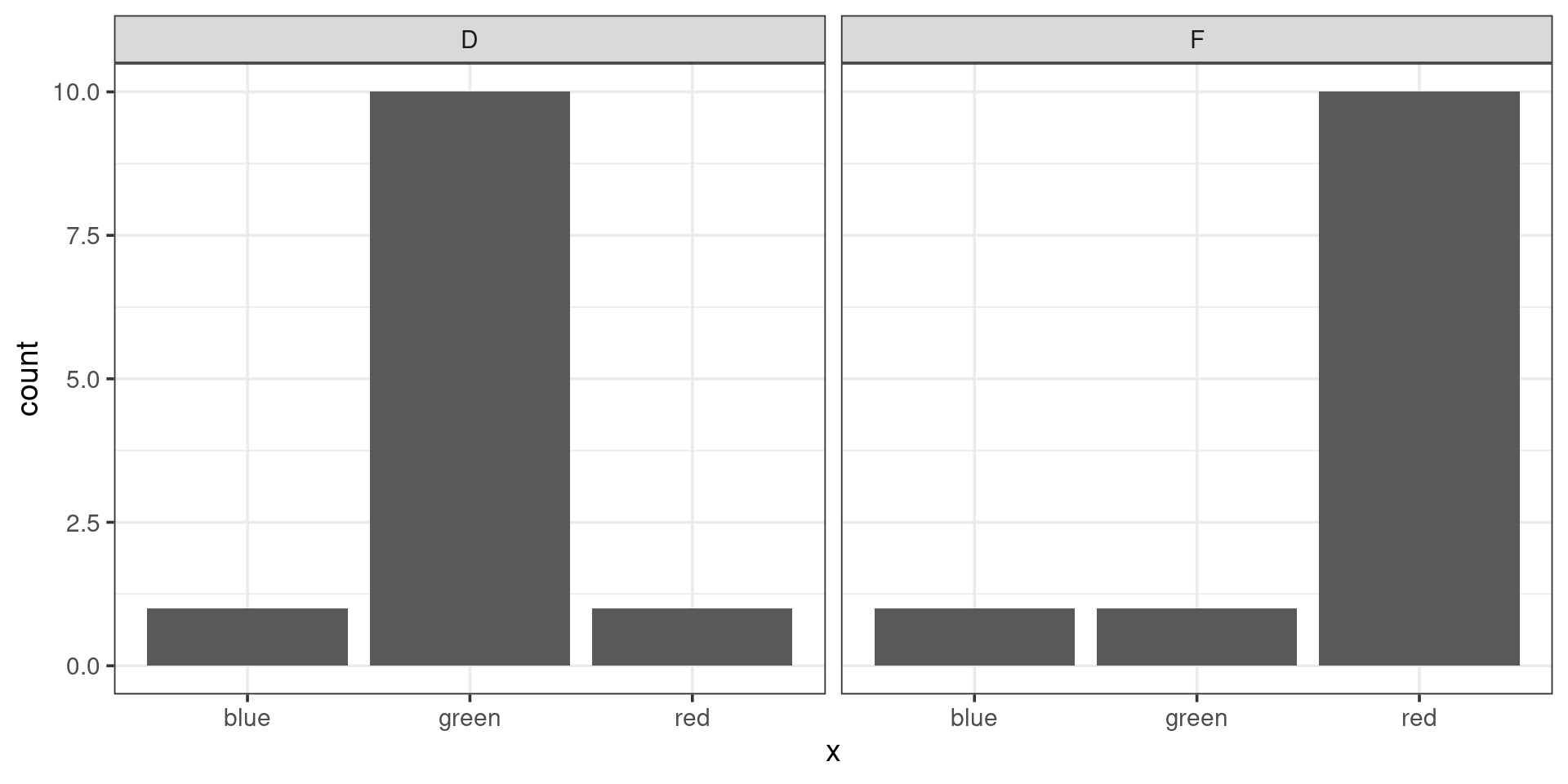
Which pair of plots would have the greatest chi-squared distance between them? (consider one of them the “observed” and the other the “expected”)

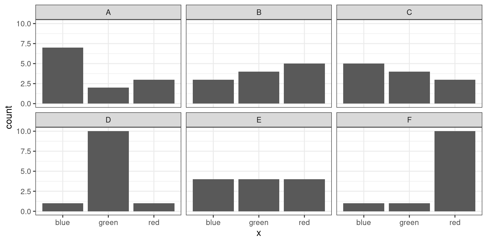
01:00

This question recalls the introduction of a new summary statistic in the notes: the chi-squared. It is used to measure the distance between two distributions of categorical variables. The pair with the highest statistic is D and F. The important mathematical intuition to have here is that the statistic adds together every squared normalized difference, so one very large difference can inflate the statistic.

Chi-squareds Compared

\[ \frac{(1-1)^2}{1} + \frac{(10 - 1)^2}{1} + \frac{(1 - 10)^2}{10} \\ 0 + 81 + \frac{81}{10} = 89.1 \]

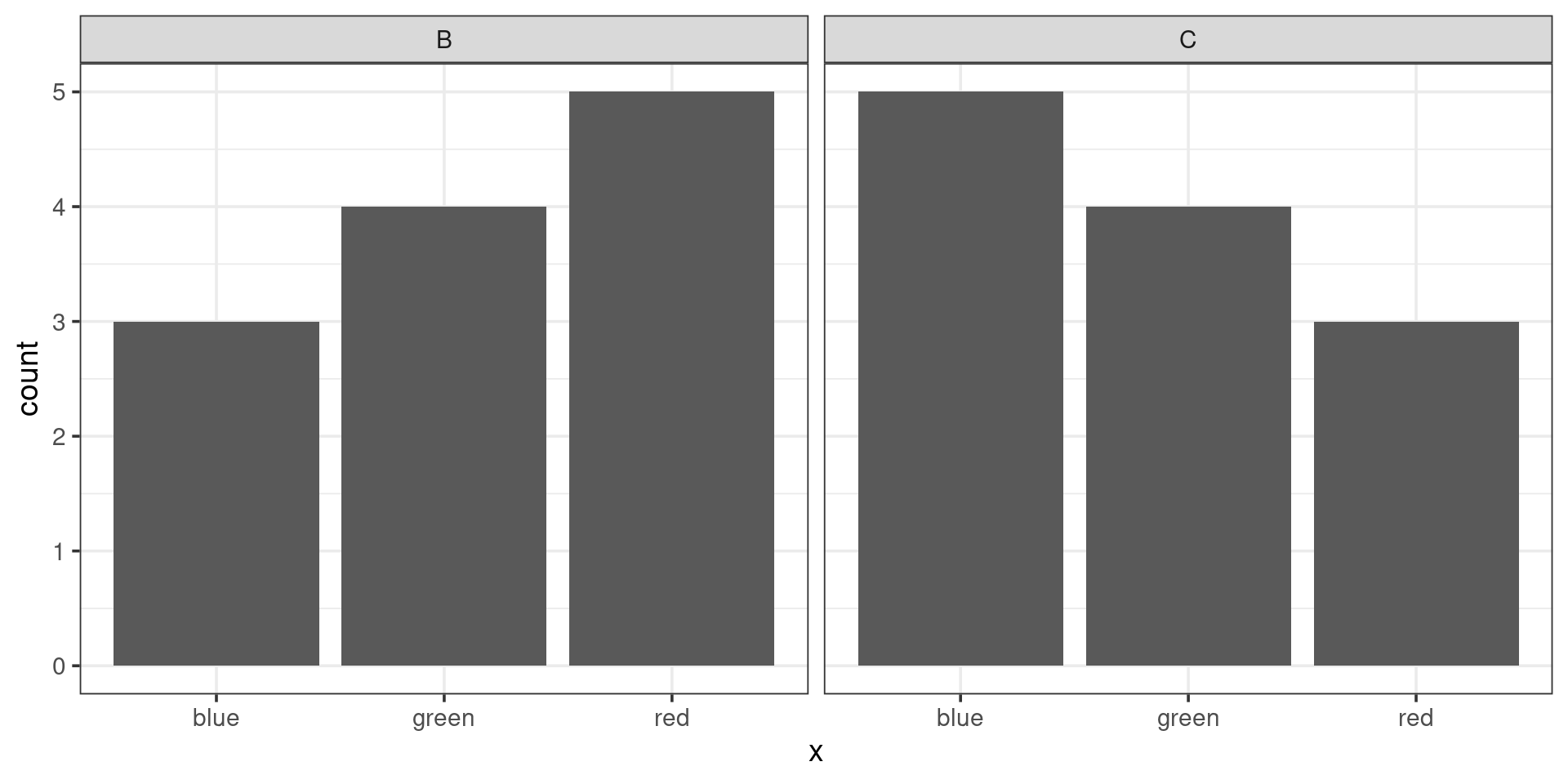
\[ \frac{(3-5)^2}{5} + \frac{(4-4)^2}{4} + \frac{(5-3)^2}{3} \\ \frac{4}{5} + 0 + \frac{4}{3} = 2.13 \]

An In-class Experiment

In order to demonstrate how to conduct a hypothesis test through simulation, we will be collecting data from this class using a poll.

You will have only 15 seconds to answer the following multiple choice question, so please get ready at pollev.com…

This sets up a discussion of how to set up a hypothesis test that p = .5.

This is based on a series of experiments that show a link between sounds and shapes in people’s minds - sharper shapes correspond to sharper sounds (k, t) and rounder shapes to rounder sounds (m, b). Read more about it here: https://en.wikipedia.org/wiki/Bouba/kiki_effect.

You conduct the experiment on the students using a poll question, then you calculate a proportion, then entertain the notion that linking names to shapes is meaningless, so people were choosing randomly, then use that to motivate the hypothesis test that p = .5.

The two shapes above have simple first names:

• Bouba
• Kiki

Which of the two names belongs to the shape on the left?

00:15

This poll everywhere question is set up to record the counts of each category and display the total number of responses in the upper right. This allows you to discuss the results either in terms of a binomial or in terms of a proportion.

Steps of a Hypothesis Test

1. Assert a model for how the data was generated (the null hypothesis)
2. Select a test statistic that bears on that null hypothesis (a mean, a proportion, a difference in means, a difference in proportions, etc).
3. Approximate the sampling distribution of that statistic under the null hypothesis (aka the null distribution)
4. Assess the degree of consistency between that distribution and the test statistic that was actually observed (either visually or by calculating a p-value)

1. The Null Hypothesis

• Let \(p_k\) be the probability that a person selects Kiki for the shape on the left.
• Let \(\hat{p}_k\) be the sample proportion of people that selected Kiki for the shape on the left.

What is a statement of the null hypothesis that corresponds to the notion the link between names and shapes is arbitrary?

01:00

2. Select a test statistic

\[\hat{p}_k = \frac{\textrm{Number who chose "Kiki"}}{\textrm{Total number of people}}\]

Note: you could also simply \(n_k\), the number of people who chose “Kiki”.

A follow-up question to ask: “For our class, what would we expect this number to be if \(p_k = .5\)?”

It should be half the number of students who responded to the poll.

3. Approximate the null distribution

Our technique: simulate data from a world in which the null is true, then calculate the test statistic on the simulated data.

Which simulation method(s) align with the null hypothesis and our data collection process?

01:00

A, C, and E all work.

Simulating the null using infer

library(tidyverse)
library(infer)

# update these based on the poll
n_k <- 40
n_b <- 20

shapes <- data.frame(name = c(rep("Kiki", n_k),
                              rep("Bouba", n_b)))

shapes |>
  specify(response = name,
          success = "Kiki") |>
  hypothesize(null = "point", p = .5) |>
  generate(reps = 1, type = "draw") |>
  calculate(stat = "prop")

1. have students open laptops and an R script to code along.
2. copy and paste the code cell from the slides into RStudio
3. replace n_k and n_b with the values from your poll.
4. “break the pipe” to show what happens at every stage.
5. run several pipelines with reps = 1 to show it changing.
6. set reps to 500 to show the full collection of p-hats.

4. Assess the consistency of the data and the null

null <- shapes |>
  specify(response = name,
          success = "Kiki") |>
  hypothesize(null = "point", p = .5) |>
  generate(reps = 500, type = "draw") |>
  calculate(stat = "prop")

obs_p_hat <- shapes |>
  specify(response = name,
          success = "Kiki") |>
  # hypothesize(null = "point", p = .5) |>
  # generate(reps = 500, type = "simulate") |>
  calculate(stat = "prop")

4. Assess the consistency of the data and the null

null |>
  visualise() +
  shade_pvalue(obs_p_hat, direction = "both")

null |>
  get_p_value(obs_p_hat, direction = "both")

The p-value

What is the proper interpretation of this p-value?

01:00

The Bouba / Kiki Effect